1. NumPy#
1. Introduction#
Numpy stands for Numerical python and it is typically imported as np
import numpy as np
The major data structure numpy provides is the array, or more accurately ndarray, and arrays can represent data in multiple Dimensions. Section 9 of this tutorial goes over several other types of data structures but we will focus on the array.
1.1: Features of an Array#
Homgeonous Data Type (Structured Arrays can have multiple data types but store data differently)
Once created size can not be changed
Must be rectangular
1.2: Array Dimensionality#
Dimension (Rank) |
Common Name |
Description |
Example Shape ( |
|---|---|---|---|
0D |
Scalar |
A single numerical value, not an array but an atomic element. |
|
1D |
Vector |
A one-dimensional array (list-like but with array properties). |
|
2D |
Matrix |
A rectangular grid of numbers with rows and columns. |
|
3D |
Tensor |
A stack of matrices, used in physics and deep learning. |
|
4D |
HyperTensor |
Higher-order tensor, used in advanced machine learning. |
|
nD |
nD Array (General) |
An array with any number of dimensions ( |
|
Array Axes#
An axes is a dimension along which data is arranged in a NumPy array and you can think of it as an indexing direction that allows you to navigate and manipulate data. Note, axis 0 is the highest ranked axes.
Dimension (Rank) |
Axes |
Description |
|---|---|---|
1D Array |
1 axis ( |
Like a Python list: a single sequence of elements. |
2D Array |
2 axes ( |
Like a table (rows and columns). |
3D Array |
3 axes ( |
Like multiple stacked tables. |
4D array Example#
Multiple experiments of the spectra of a reaction mixture where reactants concentrations are varied.
Axis |
Description |
Role in Experiment |
|---|---|---|
Axis 0 |
Experiment Number |
Separate runs where reactant concentrations vary |
Axis 1 |
Temporal Data Cube |
Absorbance values at different times |
Axis 2 |
Wavelength |
Spectral dimension (e.g., 400-700 nm) |
Axis 3 |
Absorbance at Wavelength |
Intensity values at each wavelength |
Since NumPy indexing follows axes, so you can retrieve meaningful slices from your data.
1.3 Array Properties#
Arrays use brackets like lists and in fact a 1D array looks like a list, but the array holds one block of memory while the list has pointers to multiple memory blocks.
Fixed Data Type (All elements of same data type)
Arrays are Mutable (You can change values within an array)
Fixed Size (Fixed upon creation)
Efficient Memory Usage (stores data in contiguous memory)
Vectorized Operations (supports element-wise operations that a list would require loops for)
Multi-Dimensional Support (Does not need nested structures like a list would)
2. Arrays as a Python Objects#
Table of NumPy Array Attributes#
Attribute |
Description |
|---|---|
|
Tuple of array dimensions |
|
Number of array dimensions |
|
Total number of elements in the array |
|
Data type of the array elements |
|
Size in bytes of each array element |
|
Python buffer object pointing to the array’s data |
|
Tuple of bytes to step in each dimension when traversing the array |
|
Information about the memory layout of the array |
|
Real part of the array (for complex number arrays) |
|
Imaginary part of the array (for complex number arrays) |
Table of NumPy Array Methods#
Method |
Description |
|---|---|
|
Returns a new array with a changed shape |
|
Returns a new array with axes transposed |
|
Returns a copy of the array collapsed into one dimension |
|
Cast the array to a specified data type |
|
Return a copy of the array |
|
Fill the array with a scalar value |
|
Sort an array in-place |
|
Return the maximum value along a given axis |
|
Return the minimum value along a given axis |
|
Compute the arithmetic mean along the specified axis |
Table of NumPy Functions for Arrays#
Function |
Description |
|---|---|
|
Create an array |
|
Create an array filled with zeros |
|
Create an array filled with ones |
|
Create an array with evenly spaced values within a given interval |
|
Create an array with evenly spaced numbers over a specified interval |
|
Join arrays along an existing axis |
|
Stack arrays vertically (row-wise) |
|
Stack arrays horizontally (column-wise) |
|
Split an array into multiple sub-arrays |
|
Return elements chosen from two arrays depending on condition |
3. Array Data Types#
dtype()#
In python everything has a type, which you can find with the type() function. In Numpy data also has a type function called dtype(), which like the type(), defines how much memory the object uses. The following table covers the common data types stored in a Numpy Array and it is often important to define these when creating an array.
Code |
Data Type |
Example Equivalent |
|---|---|---|
|
Boolean |
|
|
Integer (default) |
|
|
Long Integer |
|
|
Unsigned Integer |
|
|
Floating Point |
|
|
Complex Float |
|
|
Timedelta |
N/A |
|
Datetime |
N/A |
|
Object (Python objects) |
N/A |
|
String (bytes) |
Fixed-length strings |
|
Unicode String |
Fixed-length Unicode |
.astype() -changing dtypes#
import numpy as np

# Example array of long integers
arr = np.array([1733976600, 1733798400], dtype='l')

# Convert to float
arr_float = arr.astype('f8')  # Convert to float64
import numpy as np

# Example array
arr = np.array([1733976600, 1733798400], dtype='l')

# Check dtype
print(arr)
print(arr.dtype)
print(f'memory location = {id(arr)}\n')
# Convert to float
arr_float = arr.astype('f8')  # Convert to float64
print(arr_float)
print(arr_float.dtype)
print(f'memory location = {id(arr_float)}')
[1733976600 1733798400]
int64
memory location = 130959724447856

[1.7339766e+09 1.7337984e+09]
float64
memory location = 130958383798800
4. Basic Array Tasks#
4.1: Creating Arrays#
Array syntax looks like a Python list for a 1D Array in that the elements are in square brackets and separated by commas.
Array constructor (np.array())#
Creating Arrays from other python objects. In this exercise we are going to use nested python lists to create an array with the array constructor np.array().
note, an ndarray is of a single type of data, but you can use the np.array() constructor to make a structured array, which is an array with more than one data type (see section 9 below).
1D array#
import numpy as np
my_list = [1,2,3,4,5,6,7,8]
print(f"{my_list} is {type(my_list)}.")
my_1Darray=np.array(my_list)
print(f"{my_1Darray} is {type(my_1Darray)}.")
[1, 2, 3, 4, 5, 6, 7, 8] is <class 'list'>.
[1 2 3 4 5 6 7 8] is <class 'numpy.ndarray'>.
Just as a loop an be nested inside of another loop, a list can be nested inside of another list
2D array#
my_2nested_list = [[1,2],[3,4],[5,6],[7,8]]
print(f"{my_2nested_list} is {type(my_2nested_list)}.")
my_2Darray=np.array(my_2nested_list)
print(f"{my_2Darray} is {type(my_2Darray)}.")
[[1, 2], [3, 4], [5, 6], [7, 8]] is <class 'list'>.
[[1 2]
 [3 4]
 [5 6]
 [7 8]] is <class 'numpy.ndarray'>.
3D array#
my_3nested_list = [[[1,2],[3,4]],[[5,6],[7,8]]]
print(f"{my_3nested_list} is {type(my_3nested_list)}.")
my_3Darray=np.array(my_3nested_list)
print(f"{my_3Darray} is {type(my_3Darray)}.")
[[[1, 2], [3, 4]], [[5, 6], [7, 8]]] is <class 'list'>.
[[[1 2]
  [3 4]]

 [[5 6]
  [7 8]]] is <class 'numpy.ndarray'>.
np.linespace()#
generates evenly spaced numbers over a specified range.
np.linspace(start, stop, num=50, endpoint=True, retstep=False, dtype=None)
Parameter |
Description |
|---|---|
|
The starting value of the sequence (inclusive). |
|
The ending value of the sequence. By default, it is inclusive, but you can exclude it using |
|
The number of points to generate (default = 50). |
|
If |
|
If |
|
The desired NumPy data type for the output array. |
# np.linspace(): 5 evenly spaced numbers
print("linspace:", np.linspace(1, 10, num=5))
# Output: [ 1.  3.25  5.5  7.75 10. ]
linspace: [ 1. 3.25 5.5 7.75 10. ]
np.arange()#
gives evenly spaced value over a range with control of step size and data value.
np.arange(start, stop, step=1, dtype=None)
Parameter |
Description |
|---|---|
|
The starting value (inclusive). Defaults to |
|
The ending value (exclusive by default). |
|
The increment (default = |
|
The data type of the output array. If not specified, NumPy infers it automatically. |
import numpy as np

# np.arange(): Step size of 2
print("arange:", np.arange(1, 10, 2))
# Output: [1 3 5 7 9]
arange: [1 3 5 7 9]
Comparison: np.arange() vs. np.linspace()#
Feature |
|
|
|---|---|---|
Step Control |
Uses a fixed step between values. |
Uses a fixed number of points between |
Stop Inclusion |
Exclusive (default behavior). |
Inclusive (by default), unless |
Flexibility |
Good for integer-based sequences with regular spacing. |
Better for floating-point sequences with exact spacing. |
Use Case |
When you know the step size and want values to progress by that amount. |
When you know the number of points and want them distributed evenly. |
Example |
|
|
import numpy as np

# np.arange(): Step size of 2
print("arange:", np.arange(1, 10, 2))
# Output: [1 3 5 7 9]

# np.linspace(): 5 evenly spaced numbers
print("linspace:", np.linspace(1, 10, num=5))
# Output: [ 1.  3.25  5.5  7.75 10. ]
arange: [1 3 5 7 9]
linspace: [ 1.    3.25  5.5   7.75 10.  ]
np.zeros()#
This function allows you to quickly create an array filled with zeros,
np.zeros((2))
array([0., 0.])
np.zeros((3,2))
array([[0., 0.],
       [0., 0.],
       [0., 0.]])
np.zeros((4,3,2))
array([[[0., 0.],
        [0., 0.],
        [0., 0.]],

       [[0., 0.],
        [0., 0.],
        [0., 0.]],

       [[0., 0.],
        [0., 0.],
        [0., 0.]],

       [[0., 0.],
        [0., 0.],
        [0., 0.]]])
np.ones()#
np.ones((2,3,4))
array([[[1., 1., 1., 1.],
        [1., 1., 1., 1.],
        [1., 1., 1., 1.]],

       [[1., 1., 1., 1.],
        [1., 1., 1., 1.],
        [1., 1., 1., 1.]]])
4.2: Array Indexing (Introduction)#
Indexing goes along the axes from zero to “n” for an “n” dimensional array. So a 3D array would be sheet, column, row. Let’s create a 3D NumPy array representing absorbance values at different wavelengths over time for multiple experiments.
Axis 0 → Experiment number
Axis 1 → Sample Times
Axis 2 → Wavelengths
import numpy as np

# Create a 3D array: 2 experiments, 4 sample times, 3 wavelengths
data = np.array([
    [[0.12, 0.15, 0.18], [0.14, 0.17, 0.20], [0.16, 0.19, 0.22], [0.18, 0.21, 0.24]],  # Experiment 1
    [[0.22, 0.25, 0.28], [0.24, 0.27, 0.30], [0.26, 0.29, 0.32], [0.28, 0.31, 0.34]]   # Experiment 2
])

print("Shape of the array:", data.shape)  # (2, 4, 3)
print(data)
Shape of the array: (2, 4, 3)
[[[0.12 0.15 0.18]
  [0.14 0.17 0.2 ]
  [0.16 0.19 0.22]
  [0.18 0.21 0.24]]

 [[0.22 0.25 0.28]
  [0.24 0.27 0.3 ]
  [0.26 0.29 0.32]
  [0.28 0.31 0.34]]]
This array has:
2 experiments (Axis 0)
4 time steps (Axis 1)
3 wavelengths (Axis 2)
Extracting a Single Value#
To get a single absorbance value for Experiment 2, sample time 3, Wavelength 2:
value = data[1, 2, 1]  # Experiment 2 (index 1), Time step 3 (index 2), Wavelength 2 (index 1)
print("Absorbance value:", value)
Absorbance value: 0.29
Extract a 1D array#
Obtain all absorbances for the first experiment at the second time step
time_2_exp_1 = data[0, 1, :]
print(time_2_exp_1)
[0.14 0.17 0.2 ]
Extract a 2D array#
Obtain absorbance values at third wavelength for all experiments and all sample times
wavelength_3 = data[:, :, 2]
print(wavelength_3)
[[0.18 0.2  0.22 0.24]
 [0.28 0.3  0.32 0.34]]
Slice out the first experiment#
subset = data[0:1, :, :]
print(subset.shape)
print(subset)
(1, 4, 3)
[[[0.12 0.15 0.18]
  [0.14 0.17 0.2 ]
  [0.16 0.19 0.22]
  [0.18 0.21 0.24]]]
Slice out all data for second and third sample times#
subset_time = data[:, 1:3, :]
print(subset_time.shape)
print(subset_time)
(2, 2, 3)
[[[0.14 0.17 0.2 ]
  [0.16 0.19 0.22]]

 [[0.24 0.27 0.3 ]
  [0.26 0.29 0.32]]]
Summary Table#
Operation |
Code |
Output Shape |
|---|---|---|
Single Value |
|
|
1D Time Slice |
|
|
Wavelength 3 Absorbance |
|
|
First Experiment |
|
|
Time Steps 2-3 |
|
|
Every Other Wavelength |
|
|
4.3: Array Attributes#
.shape#
Gives the shape of the array
my_array=np.ones((4,3,2))
my_array.shape
(4, 3, 2)
.ndim#
Gives the number of dimensions
my_array.ndim
3
.size#
Gives total number of elements in an array
my_array.size
24
4.4: Arrays from Functions (np.fromfunction())#
You can make an array from a function, let’s create an array for the molar mass of 1-10 elements of carbon, oxygen and hydrogen.
import numpy as np
def molar_mass_grid(element_idx, atom_count):
    # Atomic masses: C=12.01, H=1.008, O=16.00
    atomic_masses = np.array([12.01, 1.008, 16.00])
    return atomic_masses[element_idx.astype(int)] * (atom_count + 1)

mass_grid = np.fromfunction(molar_mass_grid, (3,10), dtype=float)
print(mass_grid)
[[ 12.01   24.02   36.03   48.04   60.05   72.06   84.07   96.08  108.09
  120.1  ]
 [  1.008   2.016   3.024   4.032   5.04    6.048   7.056   8.064   9.072
   10.08 ]
 [ 16.     32.     48.     64.     80.     96.    112.    128.    144.
  160.   ]]
import numpy as np

# Step 1: Define the mass grid using np.fromfunction()
def molecular_mass_grid(element_idx, atom_count):
    atomic_masses = np.array([12.01, 1.008, 16.00])  # C, H, O
    return atomic_masses[element_idx.astype(int)] * (atom_count + 1)

mass_grid = np.fromfunction(molecular_mass_grid, (3, 10), dtype=float)

# Step 2: Define a function to compute molar mass
def compute_molar_mass(formula):
    # Define mapping for element index lookup
    element_indices = {'C': 0, 'H': 1, 'O': 2}

    # Parse formula into element counts
    parsed_formula = [('C', 3), ('H', 8), ('O', 1)]  # Example: C3H8O

    # Step 3: Compute molar mass
    #molar_mass = sum(mass_grid[element_indices[element], atoms - 1] for element, atoms in parsed_formula)
    molar_mass = 0  # Initialize molar mass
    for element, atoms in parsed_formula:
        element_idx = element_indices[element]  # Get index for the element
        molar_mass += mass_grid[element_idx, atoms - 1]  # Accumulate mass using array indexing

    return molar_mass

# Step 4: Compute molar mass of C3H8O (Propanol)
molar_mass_C3H8O = compute_molar_mass("C3H8O")
print(f"Molar Mass of C3H8O: {molar_mass_C3H8O:.2f} g/mol")
Molar Mass of C3H8O: 60.09 g/mol
4.5: Sorting Arrays#
axis=0: Sort along columns (vertically)
axis=1: Sort along rows (horizontally)
axis=-1: Sort along the last axis (default)
import numpy as np

arr = np.array([[3, 1, 4], [1, 5, 9], [2, 6, 5]])
print(f'original array: \n{arr}\n')
# Sort each column

print(f'sort axis 0 \n{np.sort(arr, axis=0)}\n')

# Sort each row
print(f'sort axis 1 \n {np.sort(arr, axis=1)}')
original array:
[[3 1 4]
 [1 5 9]
 [2 6 5]]

sort axis 0
[[1 1 4]
 [2 5 5]
 [3 6 9]]

sort axis 1
 [[1 3 4]
 [1 5 9]
 [2 5 6]]
4.6 Reshaping Arrays#
.reshape()#
The number of elements of the original and reshaped arrays must be the same
(3,2,4) array must be a multiple of the product of the indices
In the following we have measurements at 5 wavelengths taken 3 different times
# Simulated absorbance data (1D)
absorbance_data = np.arange(15)  # Example: 15 absorbance values
print(absorbance_data)
# Reshape into 3 time points × 5 wavelengths
absorbance_matrix = absorbance_data.reshape(3, 5)

print(absorbance_matrix)
[ 0  1  2  3  4  5  6  7  8  9 10 11 12 13 14]
[[ 0  1  2  3  4]
 [ 5  6  7  8  9]
 [10 11 12 13 14]]
.flatten()#
-convert multi-dimensional array to a 1D array
print(absorbance_matrix)
flat_matrix=absorbance_matrix.flatten()
print(flat_matrix)
[[ 0  1  2  3  4]
 [ 5  6  7  8  9]
 [10 11 12 13 14]]
[ 0  1  2  3  4  5  6  7  8  9 10 11 12 13 14]
Transpose Arrays#
Transposing a matrix swaps columns and rows. For dimensions higher than 2 you have two choices, .T and .transpose(). The former does a full transpose and completely rearranges the order, while the latter allows you to specify axes transposed
.T vs. .transpose(): Key Differences
Feature |
|
|
|---|---|---|
Works on 2D? |
Yes (swaps rows & columns) |
Yes (same as |
Works on 3D+? |
Yes (reverses all axes) |
Yes (custom axis order) |
Custom Axis Order? |
No |
Yes ( |
Effect on (2,3,4) Shape? |
➝ |
➝ Custom order (e.g., |
.T (Full Transpose)#
Full transpose
my_array=np.arange(1,25).reshape(6,4)
print(my_array)
print(f'\ntransposed array \n{my_array.T}')
[[ 1  2  3  4]
 [ 5  6  7  8]
 [ 9 10 11 12]
 [13 14 15 16]
 [17 18 19 20]
 [21 22 23 24]]

transposed array
[[ 1  5  9 13 17 21]
 [ 2  6 10 14 18 22]
 [ 3  7 11 15 19 23]
 [ 4  8 12 16 20 24]]
.transpose()#
my_array=np.arange(1,25).reshape(2,3,4)
print(my_array)
print(f'transposing rows (3) and columns(1) of 3D array \n{my_array.transpose(0,2,1)}')
[[[ 1  2  3  4]
  [ 5  6  7  8]
  [ 9 10 11 12]]

 [[13 14 15 16]
  [17 18 19 20]
  [21 22 23 24]]]
transposing rows (3) and columns(1) of 3D array
[[[ 1  5  9]
  [ 2  6 10]
  [ 3  7 11]
  [ 4  8 12]]

 [[13 17 21]
  [14 18 22]
  [15 19 23]
  [16 20 24]]]
Scenario: Kinetic Absorbance Data for a Chemical Reaction#
A spectrometer records absorbance at multiple wavelengths over several time points across different experiments (e.g., varying reagent concentrations).
This dataset is stored in a 3D NumPy array where:
Axis 0 → 3 different experiments (e.g., different NaOH concentrations).
Axis 1 → 4 different time points (e.g., 0s, 10s, 20s…).
Axis 2 → 5 different wavelengths (e.g., 400 nm, 450 nm, 500 nm…).
Goal: The chemist needs to rearrange the dataset to focus on a wavelength-first structure, where:
Axis 0 → Wavelengths
Axis 1 → Experiments
Axis 2 → Time points
This makes it easier to extract and compare spectral changes at specific wavelengths.
import numpy as np

np.random.seed(42)  # Set the seed for reproducibility

# Simulated absorbance data: (Experiments, Time Points, Wavelengths)
absorbance_data = np.random.rand(3, 4, 5)  # Shape (3, 4, 5)

print("Original Shape:", absorbance_data.shape)  # (3,4,5)
print(absorbance_data)  # Will always generate the same random values
Original Shape: (3, 4, 5)
[[[0.37454012 0.95071431 0.73199394 0.59865848 0.15601864]
  [0.15599452 0.05808361 0.86617615 0.60111501 0.70807258]
  [0.02058449 0.96990985 0.83244264 0.21233911 0.18182497]
  [0.18340451 0.30424224 0.52475643 0.43194502 0.29122914]]

 [[0.61185289 0.13949386 0.29214465 0.36636184 0.45606998]
  [0.78517596 0.19967378 0.51423444 0.59241457 0.04645041]
  [0.60754485 0.17052412 0.06505159 0.94888554 0.96563203]
  [0.80839735 0.30461377 0.09767211 0.68423303 0.44015249]]

 [[0.12203823 0.49517691 0.03438852 0.9093204  0.25877998]
  [0.66252228 0.31171108 0.52006802 0.54671028 0.18485446]
  [0.96958463 0.77513282 0.93949894 0.89482735 0.59789998]
  [0.92187424 0.0884925  0.19598286 0.04522729 0.32533033]]]
# Transpose: (Experiments, Time Points, Wavelengths) → (Wavelengths, Experiments, Time Points)
transposed_data = absorbance_data.transpose(2, 0, 1)

print("New Shape:", transposed_data.shape)  # Expected output: (5, 3, 4)
print(transposed_data)
New Shape: (5, 3, 4)
[[[0.37454012 0.15599452 0.02058449 0.18340451]
  [0.61185289 0.78517596 0.60754485 0.80839735]
  [0.12203823 0.66252228 0.96958463 0.92187424]]

 [[0.95071431 0.05808361 0.96990985 0.30424224]
  [0.13949386 0.19967378 0.17052412 0.30461377]
  [0.49517691 0.31171108 0.77513282 0.0884925 ]]

 [[0.73199394 0.86617615 0.83244264 0.52475643]
  [0.29214465 0.51423444 0.06505159 0.09767211]
  [0.03438852 0.52006802 0.93949894 0.19598286]]

 [[0.59865848 0.60111501 0.21233911 0.43194502]
  [0.36636184 0.59241457 0.94888554 0.68423303]
  [0.9093204  0.54671028 0.89482735 0.04522729]]

 [[0.15601864 0.70807258 0.18182497 0.29122914]
  [0.45606998 0.04645041 0.96563203 0.44015249]
  [0.25877998 0.18485446 0.59789998 0.32533033]]]
4.7: Merging Arrays#
Functions like np.concatenate(), np.vstack(), np.hstack(), and np.dstack() always create a new array. They do not modify the original arrays but instead return a new one that needs to be saved to a variable.
np.vstack()#
Adds arrays as new rows (along axis 0).
Requires matching number of columns.
Example: Combining Molecular Property Data Imagine we have two datasets:
Dataset 1: Molar masses of three molecules.
Dataset 2: Molar masses of three other molecules
import numpy as np

# Molecular masses (g/mol)
mass_data = np.array([[18.015],  # Water
                      [44.01],   # CO2
                      [32.00]])  # O2

# Boiling points (°C)
boiling_data = np.array([[100],  # Water
                         [-78.5], # CO2
                         [-183]]) # O2

# Stack them vertically
merged_data = np.vstack((mass_data, boiling_data))

print(merged_data)
import numpy as np

# Molecular masses (g/mol)
mass1_data = np.array([[18.015],  # Water
                      [44.01],   # CO2
                      [32.00]])  # O2

# Molecular massess (g/mol)
mass2_data = np.array([[180.16],  # Aspirin
                         [151.16], # Acetaminophen
                         [206.28]]) # Ibuprofen

# Stack them vertically
merged_data = np.vstack((mass1_data, mass2_data))

print(merged_data)
[[ 18.015]
 [ 44.01 ]
 [ 32.   ]
 [180.16 ]
 [151.16 ]
 [206.28 ]]
np.hstack()#
Adds arrays as new columns (along axis 1).
Requires matching number of rows.
Example: Combining Molecular Property Data Imagine we have two datasets:
Dataset 1: Molecular masses of three molecules.
Dataset 2: Their boiling points.
import numpy as np

# Molecular masses (g/mol)
mass_data = np.array([[18.015],  # Water
                      [44.01],   # CO2
                      [32.00]])  # O2

# Boiling points (°C)
boiling_data = np.array([[100],  # Water
                         [-78.5], # CO2
                         [-183]]) # O2
# Stack them horizontally
merged_data = np.hstack((mass_data, boiling_data))
import numpy as np

# Molecular masses (g/mol)
mass_data = np.array([[18.015],  # Water
                      [44.01],   # CO2
                      [32.00]])  # O2

# Boiling points (°C)
boiling_data = np.array([[100],  # Water
                         [-78.5], # CO2
                         [-183]]) # O2

# Stack them horizontally
merged_data = np.hstack((mass_data, boiling_data))

print(merged_data)
[[  18.015  100.   ]
 [  44.01   -78.5  ]
 [  32.    -183.   ]]
np.column_stack()#
Works like
hstack(), but is specifically designed for 1D arrays.
Example: Pairing Element Symbols with Atomic Weights
# Element symbols
elements = np.array(['H', 'O', 'C'])

# Atomic masses
atomic_masses = np.array([1.008, 16.00, 12.01])

# Combine into a structured array
merged_data = np.column_stack((elements, atomic_masses))

print(merged_data)
[['H' '1.008']
 ['O' '16.0']
 ['C' '12.01']]
np.dstack( )#
only works on 1 and 2D arrays
Results in 3d arrays
Stacking 1D arrays#
import numpy as np

a = np.array([1, 2, 3])  # Shape (3,)
b = np.array([4, 5, 6])  # Shape (3,)

stacked = np.dstack((a, b))

print("Stacked shape:", stacked.shape)  # (1, 3, 2)
print(stacked)
Stacked shape: (1, 3, 2)
[[[1 4]
  [2 5]
  [3 6]]]
Stacking 2D arrays#
a = np.array([[1, 2], [3, 4]])  # Shape (2,2)
b = np.array([[5, 6], [7, 8]])  # Shape (2,2)

stacked = np.dstack((a, b))

print("Stacked shape:", stacked.shape)  # (2, 2, 2)
print(stacked)
Stacked shape: (2, 2, 2)
[[[1 5]
  [2 6]]

 [[3 7]
  [4 8]]]
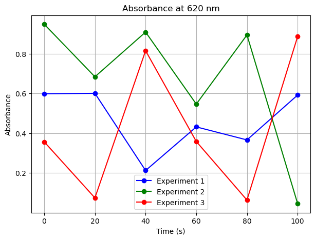
np.stack()#
For higher order arrays you need np.stack()
import numpy as np

np.random.seed(42)  # Set the seed for reproducibility

# Define common wavelength range (same for all experiments)
wavelengths = np.linspace(400, 700, 5)  # 5 wavelengths from 400 to 700 nm

# Define common time scale (to enable stacking)
common_time = np.linspace(0, 100, 6)  # 6 time points from 0s to 100s

# Simulate absorbance data (random values for illustration)
exp1 = np.random.rand(len(common_time), len(wavelengths), 1)  # Shape (6,5,1)
exp2 = np.random.rand(len(common_time), len(wavelengths), 1)  # Shape (6,5,1)
exp3 = np.random.rand(len(common_time), len(wavelengths), 1)  # Shape (6,5,1)

print("Shape of a single experiment dataset:", exp1.shape)  # (6, 5, 1)
# Stack experiments along a new axis (creating a 4D array)
spectroscopy_data = np.stack((exp1, exp2, exp3), axis=0)

print("Shape of stacked spectroscopy data:", spectroscopy_data.shape)  # (3,6,5,1)
Shape of a single experiment dataset: (6, 5, 1)
Shape of stacked spectroscopy data: (3, 6, 5, 1)
import numpy as np
import matplotlib.pyplot as plt

# Set seed for reproducibility
np.random.seed(42)

# Define common wavelength range (same for all experiments)
wavelengths = np.linspace(400, 700, 5)  # 5 wavelengths from 400 to 700 nm

# Define common time scale (to enable stacking)
common_time = np.linspace(0, 100, 6)  # 6 time points from 0s to 100s

# Simulate absorbance data (random values for illustration)
exp1 = np.random.rand(len(common_time), len(wavelengths), 1)  # Shape (6,5,1)
exp2 = np.random.rand(len(common_time), len(wavelengths), 1)  # Shape (6,5,1)
exp3 = np.random.rand(len(common_time), len(wavelengths), 1)  # Shape (6,5,1)

# Stack experiments along a new axis (creating a 4D array)
spectroscopy_data = np.stack((exp1, exp2, exp3), axis=0)

# Function to plot absorbance over time for a specific wavelength across all experiments
def plot_absorbance_at_wavelength(target_wavelength):
    """
    Plots absorbance vs time for a specific wavelength across all experiments.

    Parameters:
    target_wavelength (float): The wavelength to extract absorbance values for.
    """
    num_experiments = spectroscopy_data.shape[0]  # Number of experiments

    # Find the closest wavelength index in the wavelength array
    wavelength_idx = np.argmin(np.abs(wavelengths - target_wavelength))

    # Define experiment labels for the legend
    experiment_labels = [f'Experiment {i+1}' for i in range(num_experiments)]

    # Set up a color cycle for experiments
    colors = ['b', 'g', 'r']

    # Create figure
    plt.figure(figsize=(7, 5))

    for exp_idx in range(num_experiments):
        absorbance_values = spectroscopy_data[exp_idx, :, wavelength_idx, 0]  # Extract absorbance data

        plt.plot(common_time, absorbance_values, marker='o', linestyle='-', color=colors[exp_idx], label=experiment_labels[exp_idx])

    plt.title(f'Absorbance at {target_wavelength} nm')
    plt.xlabel('Time (s)')
    plt.ylabel('Absorbance')
    plt.legend()
    plt.grid(True)

    plt.show()

# Plot absorbance at 620 nm across all experiments
plot_absorbance_at_wavelength(620)
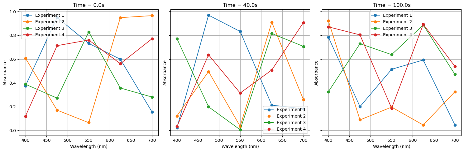
np.concatenate()#
In the above we had three experiments with the dimensions (6,5,1). We then added a fourth dimension usig np.stack() so that all three experiments are in the same array with the dimensions (3,6,5,1). We can use np.concatenate() to add a fourth experiment to the fourth dimension, giving a 4D array of shape (4,6,5,1).
# Set seed for reproducibility
np.random.seed(42)


# Simulate a new experiment (exp4) with the same shape as previous experiments
exp4 = np.random.rand(len(common_time), len(wavelengths), 1)  # Shape (6,5,1)

# Use np.concatenate() to merge exp4 along axis=0 (experiment axis)
updated_spectroscopy_data = np.concatenate((spectroscopy_data, np.expand_dims(exp4, axis=0)), axis=0)

# Print the new shape to confirm
print("Updated 4D array shape:", updated_spectroscopy_data.shape)  # Expected: (4,6,5,1)
Updated 4D array shape: (4, 6, 5, 1)
import numpy as np
import matplotlib.pyplot as plt

# Set seed for reproducibility
np.random.seed(42)

# Define common wavelength range (same for all experiments)
wavelengths = np.linspace(400, 700, 5)  # 5 wavelengths from 400 to 700 nm

# Define common time scale (to enable stacking)
common_time = np.linspace(0, 100, 6)  # 6 time points from 0s to 100s

# Simulate absorbance data (random values for illustration)
exp1 = np.random.rand(len(common_time), len(wavelengths), 1)  # Shape (6,5,1)
exp2 = np.random.rand(len(common_time), len(wavelengths), 1)  # Shape (6,5,1)
exp3 = np.random.rand(len(common_time), len(wavelengths), 1)  # Shape (6,5,1)

# Stack experiments along a new axis (creating a 4D array)
spectroscopy_data = np.stack((exp1, exp2, exp3), axis=0)

# Simulate a new experiment (exp4) with the same shape as previous experiments
exp4 = np.random.rand(len(common_time), len(wavelengths), 1)  # Shape (6,5,1)

# Use np.concatenate() to merge exp4 along axis=0 (experiment axis)
updated_spectroscopy_data = np.concatenate((spectroscopy_data, np.expand_dims(exp4, axis=0)), axis=0)

# Function to plot absorbance at different times for all experiments
def plot_absorbance_at_times(times_to_plot):
    """
    Plots absorbance vs wavelength at selected time points for all experiments.

    Parameters:
    times_to_plot (list): List of time indices to plot.
    """
    num_experiments = updated_spectroscopy_data.shape[0]  # Number of experiments

    # Define experiment labels for the legend
    experiment_labels = [f'Experiment {i+1}' for i in range(num_experiments)]

    # Use the correct Matplotlib colormap approach
    cmap = plt.colormaps.get_cmap('tab10')  # Updated approach
    colors = [cmap(i % 10) for i in range(num_experiments)]  # Ensures correct color mapping

    # Create subplots for each selected time point
    fig, axes = plt.subplots(1, len(times_to_plot), figsize=(5 * len(times_to_plot), 5), sharey=True)

    if len(times_to_plot) == 1:
        axes = [axes]  # Ensure axes is iterable for a single plot

    for ax, time_idx in zip(axes, times_to_plot):
        for exp_idx in range(num_experiments):
            absorbance_values = updated_spectroscopy_data[exp_idx, time_idx, :, 0]  # Extract absorbance data

            ax.plot(wavelengths, absorbance_values, marker='o', linestyle='-', color=colors[exp_idx], label=experiment_labels[exp_idx])

        ax.set_title(f'Time = {common_time[time_idx]:.1f}s')
        ax.set_xlabel('Wavelength (nm)')
        ax.set_ylabel('Absorbance')
        ax.legend()
        ax.grid(True)

    plt.tight_layout()
    plt.show()

# Example: Plot absorbance at selected time points (Modify as needed)
plot_absorbance_at_times([0, 2, 5])  # Plot at first, middle, and last time points
4.8: Vectorization and Broadcasting Arrays#
Vectorization#
Because of the way arrays are stored in memory you can do operations on every element within an array without having to go through a loop. If the arrays have identical shapes this is called vectorization, and this is much faster than using loops.
In the following code we have two 1D arrays with 3 elements each, one containing the numbers of carbon, hydrogen and oxygen in a molecule, and the second the molar mass of carbon, hydrogen and oxygen. Two calculate the molar mass we simply multiply the two arrays by each other.
elements = np.array(['C', 'H', 'O'])
counts = np.array([6, 12, 6])

atomic_weights_np = np.array([12.01, 1.008, 16.00])  # Order matches elements

mass_matrix = atomic_weights_np * counts
print(mass_matrix)

total_mass = np.sum(atomic_weights_np * counts)
print(total_mass)  # 180.156 g/mol
What happens is
Index 0: 6 * 12.01 = 72.06
Index 1: 12 * 1.008
Index 2: 6 * 16.00 And this is much faster than looping.
elements = np.array(['C', 'H', 'O'])
counts = np.array([6, 12, 6])

atomic_weights_np = np.array([12.01, 1.008, 16.00])  # Order matches elements
mass_matrix = atomic_weights_np * counts
print(mass_matrix)

total_mass = np.sum(atomic_weights_np * counts)
print(total_mass)  # 180.156 g/mol
[72.06  12.096 96.   ]
180.156
Broadcasting#
If the shapes do not match Numpy Broadcasts from the array with the smaller dimensions to the larger by expanding the smaller one to fit the size of the larger.
Scalar math on arrays#
becomes $\( \left[ \begin{array}{cc} 2 & 4 \\ 6 & 8 \end{array} \right] \times \left[ \begin{array}{cc} 2 & 2 \\ 2 & 2 \end{array} \right]= \left[ \begin{array}{cc} 4 & 8 \\ 12 & 16 \end{array} \right] \)$
a = np.array([[2,4], [6,8]])
b = np.array([2])
a * b
array([[ 4,  8],
       [12, 16]])
becomes $\( \left[ \begin{array}{cc} 2 & 4 \\ 6 & 8 \end{array} \right] \times \left[ \begin{array}{cc} 4 & 8 \\ 4 & 8 \end{array} \right]= \left[ \begin{array}{cc} 8 & 32 \\ 24 & 48 \end{array} \right] \)$
a = np.array([[2,4], [6,8]])
b = np.array([4,8])
a * b
array([[ 8, 32],
       [24, 64]])
4.9 Array io (saving arrays)#
You can save an array as a binary file (*.npy) or a binary compressed file (*.npz)
Save/Load a NumPy array#
import numpy as np

arr = np.array([[1.0, 2.0, 3.0], [4.0, 5.0, 6.0]])
np.save("data.npy", arr)  # Saves as binary file
loaded_arr = np.load("data.npy")
print(loaded_arr)
import numpy as np
import os

sandbox_dir = os.path.expanduser("~/sandbox/")
ndarray_npy_sbpath = os.path.join(sandbox_dir, "data.npy")

# Ensure the ~/sandbox/ directory exists
os.makedirs(sandbox_dir, exist_ok=True)

arr = np.array([[1.0, 2.0, 3.0], [4.0, 5.0, 6.0]])
np.save(ndarray_npy_sbpath, arr)  # Saves as binary file
print(arr)
[[1. 2. 3.]
 [4. 5. 6.]]
loaded_arr = np.load(ndarray_npy_sbpath)
print(loaded_arr)
[[1. 2. 3.]
 [4. 5. 6.]]
Save/Load multiple arrays#
np.savez("data.npz", arr1=arr, arr2=np.arange(10))
data = np.load("data.npz")
print(data["arr1"])  # Retrieve first array
print(data["arr2"])  # Retrieve second array
import numpy as np
import os

sandbox_dir = os.path.expanduser("~/sandbox/")
ndarray_npz_sbpath = os.path.join(sandbox_dir, "data.npz")

# Ensure the ~/sandbox/ directory exists
os.makedirs(sandbox_dir, exist_ok=True)

np.savez(ndarray_npz_sbpath, arr1=np.arange(1,25).reshape(6,4), arr2=np.arange(10))
data_files = np.load(ndarray_npz_sbpath)
print(data_files["arr1"])  # Retrieve first array
print(data_files["arr2"])  # Retrieve second array
[[ 1  2  3  4]
 [ 5  6  7  8]
 [ 9 10 11 12]
 [13 14 15 16]
 [17 18 19 20]
 [21 22 23 24]]
[0 1 2 3 4 5 6 7 8 9]
5. Random Number Generation#
The random submodule allows for a variety of random number generations. It is a very powerful tool for creating datasets to test programs with, and these can be tailored to fit different distributions.
Compare Random module with np.random submodule#
import random

# Define isotopes and their natural abundance
isotopes = ["Cl-35", "Cl-37"]
weights = [0.75, 0.25]  # Probabilities based on natural abundance

# Generate 1000 random selections
random_sample = random.choices(isotopes, weights=weights, k=1000)

# Count occurrences
cl_35_count = random_sample.count("Cl-35")
cl_37_count = random_sample.count("Cl-37")

# Print results
print(f"Using random module:")
print(f"Cl-35: {cl_35_count}, Cl-37: {cl_37_count}")
Using random module:
Cl-35: 764, Cl-37: 236
# Numpy random Submodule
import numpy as np

# Define isotopes and their probabilities
isotopes = np.array(["Cl-35", "Cl-37"])
probabilities = [0.75, 0.25]

# Generate 1000 random selections using NumPy
np_sample = np.random.choice(isotopes, size=1000, p=probabilities)

# Count occurrences using NumPy
unique, counts = np.unique(np_sample, return_counts=True)
isotope_counts = dict(zip(unique, counts))

# Print results
print("\nUsing numpy.random:")
print(f"Cl-35: {isotope_counts['Cl-35']}, Cl-37: {isotope_counts['Cl-37']}")
Using numpy.random:
Cl-35: 749, Cl-37: 251
Comparing the time we see that the numpy.random.choice is an order of magnitude faster than random.choices
import time

# Using random module
start = time.time()
random_sample = random.choices(isotopes, weights=weights, k=1_000_000)
end = time.time()
print(f"random.choices() time: {end - start:.5f} seconds")

# Using numpy.random
start = time.time()
np_sample = np.random.choice(isotopes, size=1_000_000, p=probabilities)
end = time.time()
print(f"numpy.random.choice() time: {end - start:.5f} seconds")
random.choices() time: 0.29654 seconds
numpy.random.choice() time: 0.03485 seconds
Functions and Methods in numpy.random#
Name |
Type |
Description |
|---|---|---|
|
Function |
Generates random floats uniformly distributed in [0.0, 1.0). |
|
Function |
Generates random values in a given shape from a uniform distribution over [0, 1). |
|
Function |
Returns random integers from a specified range. |
|
Function |
Randomly selects elements from a given 1D array or list. |
|
Function |
Generates random floats uniformly distributed between specified low and high values. |
|
Function |
Draws samples from a normal (Gaussian) distribution with specified mean and standard deviation. |
|
Function |
Returns samples from a standard normal distribution (mean=0, std=1). |
|
Method |
Sets the seed for reproducibility of random number generation. |
|
Class/Method |
Creates a container for managing random number generation with its own state. |
|
Method |
Returns a new instance of the default random number generator introduced in NumPy 1.17. |
|
Method |
Generates random integers over a specified range (replacement for |
|
Method |
Shuffles the elements of an array in place. |
|
Method |
Returns a permuted sequence or array without modifying the input. |
|
Function |
Draws samples from a Beta distribution. |
|
Function |
Draws samples from a Binomial distribution. |
|
Function |
Draws samples from a Poisson distribution. |
|
Function |
Draws samples from an exponential distribution. |
|
Function |
Draws samples from a Gamma distribution. |
|
Function |
Draws samples from a geometric distribution. |
np.random.seed()#
A random.seed allows you to generate the same random values when you rerun the code.
Allows reproducible data sets
Global - affects all subsequent random generation calls within a program unless another seed is set.
Works with random functions like np.random.rand() and np.random.int()
import numpy as np

# Set the seed
np.random.seed(42)

# Generate 10 random numbers to the hundredth place
random_numbers = np.round(np.random.rand(10), 2)
print(random_numbers)
[0.37 0.95 0.73 0.6 0.16 0.16 0.06 0.87 0.6 0.71]
np.random.default_rng()#
This allows you to create an independent (non global random instance). Note, the second time you call it the numbers are different because you have advanced through the seed iteration, and you need to reset the seed to start over.
import numpy as np

# First approach: The RNG advances
rng1 = np.random.default_rng(42) # seed is 42
rng2 = np.random.default_rng(99) # seed is 99

print("First call - RNG 1:", rng1.random(3))  # Advances
print("First call - RNG 2:", rng2.random(3))  # Advances

print("Second call - RNG 1:", rng1.random(3))  # Different numbers!
print("Second call - RNG 2:", rng2.random(3))  # Different numbers!

# Reset the generators
rng1 = np.random.default_rng(42)  # Reinitialize
rng2 = np.random.default_rng(99)  # Reinitialize

print("Reset and first call again - RNG 1:", rng1.random(3))  # Same as first call!
print("Reset and first call again - RNG 2:", rng2.random(3))  # Same as first call!
First call - RNG 1: [0.77395605 0.43887844 0.85859792]
First call - RNG 2: [0.50603067 0.56509163 0.51191596]
Second call - RNG 1: [0.69736803 0.09417735 0.97562235]
Second call - RNG 2: [0.97218637 0.61490314 0.5682835 ]
Reset and first call again - RNG 1: [0.77395605 0.43887844 0.85859792]
Reset and first call again - RNG 2: [0.50603067 0.56509163 0.51191596]
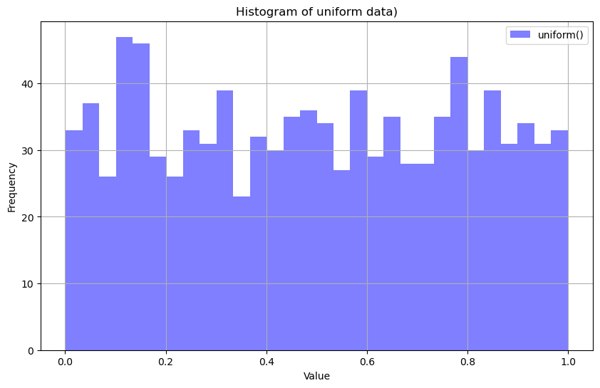
Uniform Distribution#
import numpy as np
import matplotlib.pyplot as plt

# Create an independent RNG
rng = np.random.default_rng(42)

# Generate 1000 random numbers from uniform distribution
uniform_data = rng.uniform(size=1000)


# Create a histogram plot
plt.figure(figsize=(10, 6))

# Plot uniform distribution histogram
plt.hist(uniform_data, bins=30, alpha=0.5, color='blue', label="uniform()")


# Labels and title
plt.xlabel("Value")
plt.ylabel("Frequency")
plt.title("Histogram of uniform data)")
plt.legend()
plt.grid(True)

# Show the histogram
plt.show()
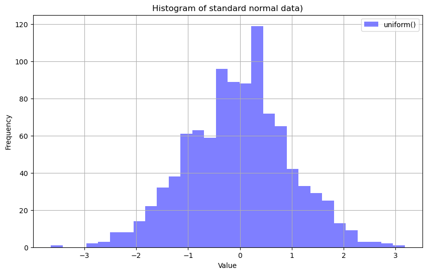
import numpy as np
import matplotlib.pyplot as plt

# Create an independent RNG
rng = np.random.default_rng(42)

# Generate 1000 random numbers from uniform distribution
standard_normal_data = rng.standard_normal(size=1000)


# Create a histogram plot
plt.figure(figsize=(10, 6))

# Plot uniform distribution histogram
plt.hist(standard_normal_data, bins=30, alpha=0.5, color='blue', label="uniform()")


# Labels and title
plt.xlabel("Value")
plt.ylabel("Frequency")
plt.title("Histogram of standard normal data)")
plt.legend()
plt.grid(True)

# Show the histogram
plt.show()
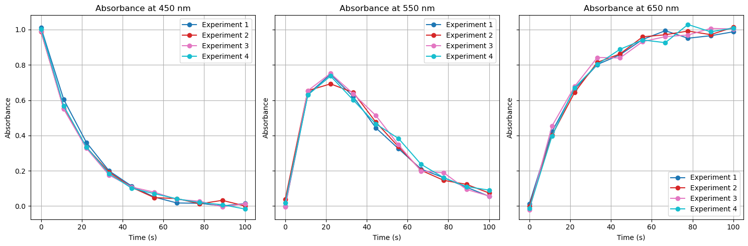
Inserting noise into an equation.
import numpy as np
import matplotlib.pyplot as plt

# Set seed for reproducibility
np.random.seed(42)

# Define wavelengths for R, I, and P
wavelengths = np.array([450, 550, 650])  # nm

# Define common time scale (10 points over 100s)
common_time = np.linspace(0, 100, 10)

# Define the number of experiments
num_experiments = 4

# Function to simulate reaction kinetics: R → I → P
def reaction_profiles(time):
    """
    Simulates reaction kinetics:
    - R (Reactant) decays exponentially.
    - I (Intermediate) forms, then decays as P forms.
    - P (Product) forms as I decays.
    """
    R = np.exp(-0.05 * time)  # Exponential decay for R
    I = (time * np.exp(-0.05 * time)) / 10  # Intermediate formation & decay
    P = (1 - np.exp(-0.05 * time))  # Product formation

    return np.array([R, I, P]).T  # Transpose to match (time, species)

# Initialize a NumPy array to store absorbance data (4D array)
# Shape: (Experiments, Time, Wavelengths, 1)
absorbance_data = np.zeros((num_experiments, len(common_time), len(wavelengths), 1))

# Generate data for each experiment
for exp_idx in range(num_experiments):
    reaction_data = reaction_profiles(common_time)  # Get kinetic profiles

    # Introduce slight experimental variations using a random factor
    noise = np.random.normal(0, 0.02, reaction_data.shape)  # Small noise added
    absorbance_data[exp_idx, :, :, 0] = reaction_data + noise  # Store data

# Function to plot absorbance vs time at selected wavelengths
def plot_absorbance_at_wavelengths():
    """
    Plots absorbance vs time for selected wavelengths (450nm, 550nm, 650nm),
    representing Reactant, Intermediate, and Product formation.
    """
    experiment_labels = [f'Experiment {i+1}' for i in range(num_experiments)]
    colors = plt.cm.tab10(np.linspace(0, 1, num_experiments))  # Assign colors

    # Create subplots for each wavelength
    fig, axes = plt.subplots(1, len(wavelengths), figsize=(15, 5), sharey=True)

    for ax, wavelength_idx in zip(axes, range(len(wavelengths))):
        for exp_idx in range(num_experiments):
            absorbance_values = absorbance_data[exp_idx, :, wavelength_idx, 0]  # Extract data

            ax.plot(common_time, absorbance_values, marker='o', linestyle='-',
                    color=colors[exp_idx], label=experiment_labels[exp_idx])

        ax.set_title(f'Absorbance at {wavelengths[wavelength_idx]} nm')
        ax.set_xlabel('Time (s)')
        ax.set_ylabel('Absorbance')
        ax.legend()
        ax.grid(True)

    plt.tight_layout()
    plt.show()

# Plot absorbance at 450nm, 550nm, and 650nm
plot_absorbance_at_wavelengths()
# Show data of second experiment
absorbance_data[1, :, :, 0]
array([[ 9.87965868e-01,  3.70455637e-02, -2.69944495e-04],
       [ 5.52599202e-01,  6.53954699e-01,  4.01829706e-01],
       [ 3.33370260e-01,  6.92346570e-01,  6.44243291e-01],
       [ 1.92812828e-01,  6.44354674e-01,  8.14551763e-01],
       [ 1.06055058e-01,  4.75613585e-01,  8.62061537e-01],
       [ 4.77796399e-02,  3.36212358e-01,  9.58965921e-01],
       [ 4.25463591e-02,  2.02565819e-01,  9.70807686e-01],
       [ 1.27664301e-02,  1.45657704e-01,  9.91765450e-01],
       [ 3.23636189e-02,  1.23013411e-01,  9.71472021e-01],
       [ 5.53699482e-04,  7.40047386e-02,  1.01277296e+00]])
# Show first four temporal measurements of third experiment
absorbance_data[2, 0:4, :, 0]
array([[ 0.99041652, -0.00371318, -0.0221267 ],
       [ 0.54982929,  0.65375432,  0.45337138],
       [ 0.32775279,  0.75161063,  0.67803973],
       [ 0.17597321,  0.63681325,  0.84188513]])
# Show the decay of the first experiment
absorbance_data[0, :, 0, 0]
array([1.00993428e+00, 6.04214018e-01, 3.60777244e-01, 1.99726804e-01,
       1.13207269e-01, 5.09307734e-02, 1.75135118e-02, 1.59525497e-02,
       8.55973967e-04, 1.42519074e-02])
#Find the values of the reactant and product when the intermediate is max.
print(absorbance_data.shape)
# Find the time index where Intermediate (I) is max for each experiment
max_I_indices = np.argmax(absorbance_data[:, :, 1, 0], axis=1)  # I at index 1 (550 nm)

# Extract corresponding R (450 nm) and P (650 nm) values
R_at_max_I = absorbance_data[np.arange(num_experiments), max_I_indices, 0, 0]  # R at 450nm
P_at_max_I = absorbance_data[np.arange(num_experiments), max_I_indices, 2, 0]  # P at 650nm

# Print results
for exp_idx in range(num_experiments):
    time_at_max_I = common_time[max_I_indices[exp_idx]]
    print(f"Experiment {exp_idx+1}:")
    print(f"  Time at max I: {time_at_max_I:.2f} s")
    print(f"  R (450nm) at max I: {R_at_max_I[exp_idx]:.3f}")
    print(f"  P (650nm) at max I: {P_at_max_I[exp_idx]:.3f}\n")
(4, 10, 3, 1)
Experiment 1:
  Time at max I: 22.22 s
  R (450nm) at max I: 0.361
  P (650nm) at max I: 0.661

Experiment 2:
  Time at max I: 22.22 s
  R (450nm) at max I: 0.333
  P (650nm) at max I: 0.644

Experiment 3:
  Time at max I: 22.22 s
  R (450nm) at max I: 0.328
  P (650nm) at max I: 0.678

Experiment 4:
  Time at max I: 22.22 s
  R (450nm) at max I: 0.335
  P (650nm) at max I: 0.671
6. Masks#
A mask is a way of filtering data based on a condition.
Instead of looping through a dataset and using
ifstatements, we can use a Boolean mask to select specific values efficiently.
In NumPy, masks are frequently used for filtering arrays.
.nonzero()#
nonzero() returns the indices of elements that are non-zero (or True for boolean arrays). For a 1D array, it returns a tuple containing a single array of indices. For multi-dimensional arrays, it returns a tuple of arrays, one for each dimension.
import numpy as np

# Define the array
darray = np.array([3, 1, 8, -8, 2, 8])

# Create a boolean mask where values equal to 8 are True
mask = (darray == 8)
print("Mask:", mask)  # [False False  True False False  True]

# Use nonzero() to find indices where mask is True
print("nonzero() result:", mask.nonzero())  # returns a tuple of arrays
print("Extracted indices:", mask.nonzero()[0])  # extract the first array from the tuple

# Separate analysis of the types
nonzero_result = mask.nonzero()
print("nonzero_result:", nonzero_result)  # (array([2, 5]),)
print("type of nonzero_result:", type(nonzero_result))  # <class 'tuple'>
print("type of nonzero_result[0]:", type(nonzero_result[0]))  # <class 'numpy.ndarray'>
Mask: [False False  True False False  True]
nonzero() result: (array([2, 5]),)
Extracted indices: [2 5]
nonzero_result: (array([2, 5]),)
type of nonzero_result: <class 'tuple'>
type of nonzero_result[0]: <class 'numpy.ndarray'>
Example: Finding Temperatures Above a Threshold
import numpy as np

# Temperature readings in °C
temperatures = np.array([20, 25, 30, 15, 10, 35, 40])

# Mask for temperatures above 25°C
high_temps = temperatures > 25
print(high_temps)  # [False False  True False False  True  True]

# Use the mask to filter values
filtered_temps = temperatures[high_temps]
print(filtered_temps)  # [30 35 40]
Why is this useful?
Instead of writing a loop with an
ifstatement, we filter data in a single operation.Faster execution for large datasets.
Useful for analyzing experimental datasets (e.g., selecting only high-energy molecules).
Why NumPy Handles True Boolean Masks#
Boolean Indexing
NumPy allows direct indexing using a Boolean array (mask), which is not possible with standard lists.
Example:
import numpy as np
arr = np.array([10, 15, 20, 25])
mask = arr > 15  # [False, False, True, True]
print(arr[mask])  # Output: [20 25]
This directly filters elements based on the mask.
Lists don’t support this; you’d need a list comprehension instead.
Performance Optimization
NumPy operates at C-level speed under the hood, making Boolean masks much faster than loops or comprehensions in pure Python.
Logical Operations on Masks
You can combine conditions efficiently using NumPy’s element-wise operations:
mask = (arr > 10) & (arr < 25)  # Using bitwise AND for multiple conditions
print(arr[mask])
Standard lists require multiple loops or conditions inside a comprehension.
import numpy as np

# Temperature readings in °C
temperatures = np.array([20, 25, 30, 15, 10, 35, 40])

# Mask for temperatures above 25°C
high_temps = temperatures > 25
print(high_temps)  # [False False  True False False  True  True]

# Use the mask to filter values
filtered_temps = temperatures[high_temps]
print(filtered_temps)  # [30 35 40]
[False False  True False False  True  True]
[30 35 40]
random mask (the following will print between 0 and 10 values that were generated as true
atomic_numbers = np.array([1, 2, 3, 4, 5, 6, 7, 8, 9, 10])
random_mask = np.random.randint(0, 2, size=10, dtype=bool)  # Random 0/1 mask
selected_data = atomic_numbers[random_mask]
print(selected_data)  # Random subset of elements
[2 4 5 6 7]
.where#
import numpy as np
data = np.array([3,1,8,-8,2,8])
mask = np.where(data == 8, np.arange(np.size(data)), 0)
print(mask)
[0 0 2 0 0 5]
8. Missing Data#
IEEE NaN (Not a Number)#
IEEE standard for floating point arithmetic.
Represents the absence of a valid numerical value in floating point systems
Using Boolean Masks for NaN#
import numpy as np

arr = np.array([1.0, 2.0, np.nan, 4.0, 5.0])
print(arr)
[ 1. 2. nan 4. 5.]
nan_mask = np.isnan(arr)
print(nan_mask)
[False False True False False]
nan_mask = ~np.isnan(arr)
print(nan_mask)
[ True True False True True]
The ~ is the Bitwise NOT operator and inverts the boolean mask
~inverts the Boolean mask:True→FalseFalse→True
arr_no_nan = arr[~np.isnan(arr)]
print(arr_no_nan)
[1. 2. 4. 5.]
9. NumPy Statistics#
Function |
Description |
Example |
|---|---|---|
|
Calculates the arithmetic mean |
|
|
Calculates the median (middle value) |
|
|
Calculates the standard deviation |
|
|
Calculates the variance |
|
|
Finds the minimum value |
|
|
Finds the maximum value |
|
|
Calculates the qth percentile |
|
|
Calculates the sum of all elements |
|
|
Calculates the product of all elements |
|
|
Calculates the cumulative sum |
|
|
Calculates the cumulative product |
|
|
Returns the index of the minimum value |
|
|
Returns the index of the maximum value |
|
|
Range of values (max - min) |
|
10. Numpy NaN Statistics#
Function |
Description |
Example |
|---|---|---|
|
Maximum value, ignoring NaNs |
|
|
Minimum value, ignoring NaNs |
|
|
Arithmetic mean, ignoring NaNs |
|
|
Median value, ignoring NaNs |
|
|
Sum of elements, ignoring NaNs |
|
|
Standard deviation, ignoring NaNs |
|
|
Variance, ignoring NaNs |
|
|
Product of elements, ignoring NaNs |
|
|
Cumulative sum, ignoring NaNs |
|
|
Cumulative product, ignoring NaNs |
|
|
Compute percentiles, ignoring NaNs |
|
|
Compute quantiles, ignoring NaNs |
|
12. Other Numpy DataTypes#
besides ndarray there are several other datatypes provided by the numpy package
9.1: Structured arrays (np.array)#
Allows defining heterogeneous data types .
Example:
# Define a structured dtype with multiple fields
dtype = [('name', 'U10'), ('mass', 'f4'), ('charge', 'i4')]

# Create a structured array with different field types
structured_arr = np.array([
    ('Electron', 9.11e-31, -1),
    ('Proton', 1.67e-27, +1)
], dtype=dtype)

print(structured_arr)
print(type(structured_arr))  # <class 'numpy.ndarray'>
[('Electron', 9.11e-31, -1) ('Proton', 1.67e-27,  1)]
<class 'numpy.ndarray'>
How Are Structured Arrays Different from Regular ndarrays?#
Feature |
Regular |
Structured Array ( |
|---|---|---|
Data Type |
Homogeneous ( |
Heterogeneous ( |
Row Access |
Indexed by number ( |
Indexed by number ( |
Column Access |
Not supported natively |
Accessed by field names ( |
Resemblance to DataFrames? |
No |
Yes (similar to structured tables) |
9.2: Masked arrays (np.ma.array)#
A subclass of
ndarraythat allows elements to be masked (ignored) in computations.Useful for handling missing or invalid data without affecting computations.
Example:
import numpy as np
a = np.ma.array([1, 2, 3, 4], mask=[False, True, False, False])
print(a.mean())  # Ignores masked elements
9.3: Record Arrays (np.recarray)#
A variation of structured arrays with attribute-style access. Example: rec = np.rec.array([(‘Hydrogen’, 1.008), (‘Oxygen’, 16.00)], dtype=[(‘element’, ‘U10’), (‘mass’, ‘f4’)]) print(rec.element) # Access column as an attribute
Acknowledgements#
This content was developed with assistance from Perplexity AI and Chat GPT. Multiple queries were made during the Fall 2024 and the Spring 2025.