8. SciPy

1. Introduction

SciPy is built on NumPy and offers features such as numerical integration optimization, signal processing and statistical modeling through a toolbox of scientific subpackages

Subpackage	Description
scipy.integrate	Numerical integration (quad, dblquad, odeint, solve_ivp)
scipy.optimize	Optimization algorithms and root finding
scipy.interpolate	Interpolation of functions and data
scipy.fft	Fast Fourier Transforms (replaces older scipy.fftpack)
scipy.linalg	Linear algebra (built on NumPy but more advanced features)
scipy.signal	Signal processing (filters, convolution, transfer functions)
scipy.sparse	Sparse matrix representations and operations
scipy.spatial	Spatial algorithms (KD-trees, distances, nearest neighbors)
scipy.stats	Statistical distributions, tests, and descriptive stats
scipy.constants	Physical and mathematical constants
scipy.ndimage	Multidimensional image processing
scipy.io	Input/output for formats like MATLAB, WAV, etc.
scipy.cluster	Clustering algorithms (k-means, hierarchy)

2. SciPy Constants

Symbol	Value	Meaning
N_A	6.02214076e+23 mol^-1	Avogadro constant
k	1.380649e-23 J K^-1	Boltzmann constant
R	8.314462618 J mol^-1 K^-1	Molar gas constant
F	96485.33212 C mol^-1	Faraday constant
e	1.602176634e-19 C	Elementary charge
m_e	9.1093837015e-31 kg	Electron mass
m_p	1.67262192369e-27 kg	Proton mass
m_n	1.67492749804e-27 kg	Neutron mass
h	6.62607015e-34 J s	Planck constant
c	299792458.0 m s^-1	Speed of light in vacuum
epsilon_0	8.8541878128e-12 F m^-1	Vacuum electric permittivity
mu_0	1.25663706212e-06 N A^-2	Vacuum magnetic permeability
alpha	0.0072973525693	Fine-structure constant
a_0	5.29177210903e-11 m	Bohr radius
E_h	4.3597447222071e-18 J	Hartree energy
G	6.67430e-11 m^3 kg^-1 s^-2	Gravitational constant
g	9.80665 m s^-2	Standard acceleration due to gravity
atm	101325.0 Pa	Standard atmosphere
bar	100000.0 Pa	Bar (unit of pressure)

This table includes some of the most commonly used physical constants in chemistry, along with their symbols, values, and meanings. The values are taken from the SciPy constants module, which uses the 2018 CODATA recommended values.

#from my_packages import my_pack
#print(my_pack.__file__)

from scipy import constants
#from my_pack import my_fun
#dir(constants)
#my_fun.scrollable_box(dir(constants), height='150px')

from scipy import constants

constants_list = []
for name in dir(constants):
    if name.startswith('__'):
        continue
    val = getattr(constants, name)
    if isinstance(val, (int, float)):
        constants_list.append(f"{name}: {val}")

from scipy.constants import physical_constants

phys_list = []
for name, (value, unit, _) in sorted(physical_constants.items()):
    phys_list.append(f"{name}: {value} {unit}")

3. Scipy.integrate

Function/Method	Description
quad(func, a, b[, args, full_output, …])	Compute a definite integral
dblquad(func, a, b, gfun, hfun[, args, …])	Compute a double integral
tplquad(func, a, b, gfun, hfun, qfun, rfun[, …])	Compute a triple integral
nquad(func, ranges[, args, opts, full_output])	Integration over multiple variables
fixed_quad(func, a, b[, args, n])	Compute a definite integral using fixed-order Gaussian quadrature
quadrature(func, a, b[, args, tol, rtol, …])	Compute a definite integral using fixed-tolerance Gaussian quadrature
romberg(function, a, b[, args, tol, rtol, …])	Romberg integration of a callable function or method
quad_explain([points, weights, a, b, …])	Print extra information about integrate.quad() parameters and returns
newton_cotes(rn[, equal])	Return weights and error coefficient for Newton-Cotes integration
IntegrationWarning	Warning on issues during integration
odeint(func, y0, t[, args, Dfun, col_deriv, …])	Integrate a system of ordinary differential equations
ode(f[, jac])	A generic interface class to numeric integrators
complex_ode(f[, jac])	A wrapper of ode for complex systems
solve_ivp(fun, t_span, y0[, method, t_eval, …])	Solve an initial value problem for a system of ODEs
RK23(fun, t0, y0, t_bound[, max_step, rtol, …])	Explicit Runge-Kutta method of order 3(2)
RK45(fun, t0, y0, t_bound[, max_step, rtol, …])	Explicit Runge-Kutta method of order 5(4)
DOP853(fun, t0, y0, t_bound[, max_step, …])	Explicit Runge-Kutta method of order 8
Radau(fun, t0, y0, t_bound[, max_step, …])	Implicit Runge-Kutta method of Radau IIA family of order 5
BDF(fun, t0, y0, t_bound[, max_step, rtol, …])	Implicit method based on backward-differentiation formulas
LSODA(fun, t0, y0, t_bound[, first_step, …])	Adams/BDF method with automatic stiffness detection and switching
solve_bvp(fun, bc, x, y[, p, S, fun_jac, …])	Solve a boundary-value problem for a system of ODEs

scipy.integrate.quad() Adaptive Quadrature (integration technique)

Adaptive quadrature is a numerical integration technique that automatically adjusts its approach based on the behavior of the function being integrated. It uses smaller step sizes in regions where the function is more complex or rapidly changing, and larger step sizes where the function is smoother.

Argument	Type	Description
func	callable	The function to integrate (must take a float and return a float).
a	float	Lower limit of integration.
b	float	Upper limit of integration.
args	tuple	Extra arguments passed to func.
full_output	bool	If True, return additional output info.
epsabs	float	Absolute error tolerance (default: 1.49e-8).
epsrel	float	Relative error tolerance (default: 1.49e-8).
limit	int	Max number of subintervals (default: 50).
points	list of float	Points to avoid singularities or help convergence (e.g., discontinuities).
weight	str (optional)	Weighting function for weighted integrals (e.g., ‘cos’, ‘sin’).
wvar	float	Variable for the weighting function.
wopts	tuple	Optional parameters for weighting function.
maxp1	int	Max number of Chebyshev moments.
limlst	int	Max number of cycles for oscillatory weights.

\[ \int_{0}^{2} x^2 \, dx \]

This equation represents the definite integral of the function f(x) = x² over the interval [0, 2]. The result of this integration is 8/3 or approximately 2.667. quad() returns a tuple as the answer with the second part being the error estimate

 from scipy.integrate import quad
def func(x):
    return x**2

quad(func, 0,2)

(2.666666666666667, 2.960594732333751e-14)

\[ \int_{-1}^{1} \frac{1}{|1-4x^2|} \, dx \]

This equation represents the definite integral of the function f(x) = 1/|1-4x²| over the interval [-1, 1].

A few notes about this integral:

1. The absolute value in the denominator (|1-4x²|) ensures that the function is defined for all x in the interval [-1, 1].

2. This integral has vertical asymptotes (singularity) at x = ±1/2, where the denominator becomes zero.

3. Due to the singularity, this integral is improper and may not converge in the usual sense. Special techniques or numerical methods might be needed to evaluate it. The following code uses a lambda function, which is a short, anonymous function in Python. It’s useful when you want to define a function on the fly — especially when passing it to another function like quad.

import numpy as np
f = lambda x: 1 / np.sqrt(np.abs(1-4*x**2))
quad(f,-1,1)

This is equivalent to:

def f(x):
    return 1 / np.sqrt(np.abs(1 - 4 * x**2))

import numpy as np
f = lambda x: 1 / np.sqrt(np.abs(1-4*x**2))
quad(f,-1,1)

/tmp/ipykernel_67240/1021973711.py:2: RuntimeWarning: divide by zero encountered in scalar divide
  f = lambda x: 1 / np.sqrt(np.abs(1-4*x**2))

(inf, inf)

To handle the singularity we use the keyword argument points=[-0.5,0.5] and quad() splits the integration around those points

f = lambda x: 1 / np.sqrt(np.abs(1-4*x**2))
quad(f,-1,1, points=[-0.5,0.5])

(2.8877542237184186, 3.632489864457966e-10)

Gausian integral

\[ \int_{-\infty}^{\infty} e^{-x^2} \, dx = \sqrt{\pi}\]

This improper integral represents the Gaussian (bell curve) and is a fundamental integral in mathematics and physics, particularly in probability theory and statistics.

The Python code quad(lambda x: np.exp(-(x**2)), -np.inf, np.inf) uses SciPy’s quad function to numerically evaluate this improper integral from negative infinity to positive infinity.

Interestingly, the exact value of this integral is known to be \(\sqrt{\pi}\), which is approximately 1.77245385090551603.

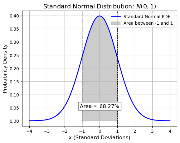
Probability Density Function (PDF)

\[ f(x) = \frac{1}{\sqrt{2\pi}} e^{-x^2 / 2} \]

This function is chosen specifically so that the total area under the curve is 1, meaning:

\[ \int_{-\infty}^{\infty} f(x) \, dx = \int_{-\infty}^{\infty} \frac{1}{\sqrt{2\pi}} e^{-x^2/2} \, dx = 1 \]

import numpy as np
import matplotlib.pyplot as plt
from scipy.stats import norm

# Define the range for x
x = np.linspace(-4, 4, 500)
y = norm.pdf(x)  # Standard normal PDF

# Plot the standard normal distribution curve
plt.plot(x, y, label='Standard Normal PDF', color='blue', linewidth=2)

# Define the interval: from -1 to +1
x_fill = np.linspace(-1, 1, 300)
y_fill = norm.pdf(x_fill)

# Shade the area between -1 and 1
plt.fill_between(x_fill, y_fill, alpha=0.4, color='gray', label='Area between -1 and 1')

# Compute the area (probability) using the CDF
area = norm.cdf(1) - norm.cdf(-1)  # P(-1 < X < 1)
area_percent = area * 100

# Add vertical lines for -1 and +1
plt.axvline(-1, color='black', linestyle='--', linewidth=1)
plt.axvline(1, color='black', linestyle='--', linewidth=1)

# Add annotation with computed area
plt.text(0, 0.05, f'Area ≈ {area_percent:.2f}%', ha='center', fontsize=12, bbox=dict(facecolor='white', edgecolor='gray'))

# Titles and labels
plt.title('Standard Normal Distribution: $N(0,1)$', fontsize=14)
plt.xlabel('x (Standard Deviations)', fontsize=12)
plt.ylabel('Probability Density', fontsize=12)
plt.legend()
plt.grid(True)
plt.show()

From Gaussian Distribution to PDF:

run the following code cell

import numpy as np
import matplotlib.pyplot as plt
from scipy.integrate import quad

# Define x range
x = np.linspace(-5, 5, 500)

# Define all three functions
f1 = np.exp(-x**2)                              # Original Gaussian
f2 = np.exp(-x**2 / 2)                          # Stretched version
f3 = (1 / np.sqrt(2 * np.pi)) * f2              # Normalized standard normal PDF

# Compute areas under each curve
area_f1, _ = quad(lambda x: np.exp(-x**2), -np.inf, np.inf)
area_f2, _ = quad(lambda x: np.exp(-x**2 / 2), -np.inf, np.inf)
area_f3, _ = quad(lambda x: (1 / np.sqrt(2 * np.pi)) * np.exp(-x**2 / 2), -np.inf, np.inf)

# Plot each function
plt.plot(x, f1, label=rf'$e^{{-x^2}}$ (Area ≈ {area_f1:.3f})', linewidth=2)
plt.plot(x, f2, label=rf'$e^{{-x^2/2}}$ (Area ≈ {area_f2:.3f})', linewidth=2, linestyle='--')
plt.plot(x, f3, label=rf'$\frac{{1}}{{\sqrt{{2\pi}}}} e^{{-x^2/2}}$ (Area ≈ {area_f3:.3f})',
         linewidth=2, linestyle=':')

# Fill under the normalized PDF
plt.fill_between(x, f3, alpha=0.2, color='green')

# Add titles, labels, and legend
plt.title('From Gaussian Integral to Normalized PDF', fontsize=14)
plt.xlabel('x')
plt.ylabel('f(x)')
plt.grid(True)
plt.legend()
plt.tight_layout()
plt.show()

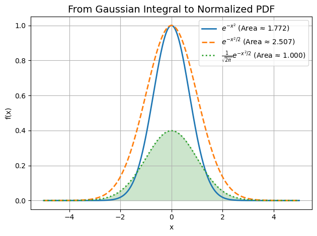
• Blue (solid): \( e^{-x^2} \) — the classic Gaussian integral. Area ≈ √π ≈ 1.772

• Orange (dashed): \( e^{-x^2/2} \) — stretched version. Area ≈ √(2π) ≈ 2.506

• Green (dotted): \( \frac{1}{\sqrt{2\pi}} e^{-x^2/2} \) — normalized PDF. Area ≈ 1.000

Particle in a Box

The “particle in a box” is the generic name for the quantum model where a particle is confined to a finite region of space with infinite potential outside. The dimensionality defines the specific case:

• 1D box: Particle can only move along one axis. $\( \psi_n(x) = \sqrt{\frac{2}{L}} \sin\left(\frac{n\pi x}{L}\right) \)$ → Use scipy.integrate.quad()

• 2D box (square well): Particle moves in a 2D rectangle or square. $\( \psi_{n,m}(x,y) = \sqrt{\frac{4}{L_x L_y}} \sin\left(\frac{n\pi x}{L_x}\right) \sin\left(\frac{m\pi y}{L_y}\right) \)$ → Use scipy.integrate.dblquad()

• 3D box (cube or rectangular prism): Now you add the z-dimension. $\( \psi_{n,m,l}(x,y,z) = \sqrt{\frac{8}{L_x L_y L_z}} \sin\left(\frac{n\pi x}{L_x}\right) \sin\left(\frac{m\pi y}{L_y}\right) \sin\left(\frac{l\pi z}{L_z}\right) \)$ → Use scipy.integrate.tplquad()

1D Box

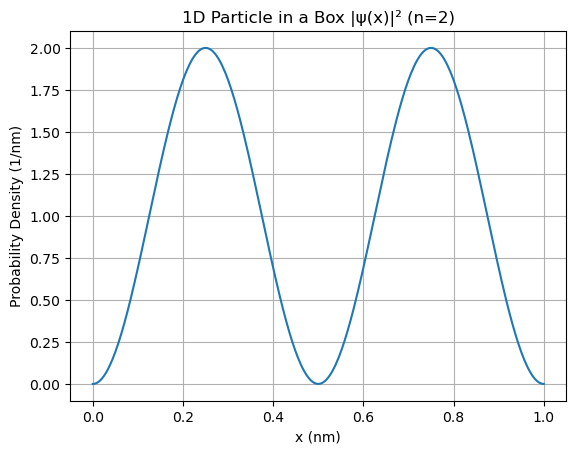
The wavefunction is: $\( \psi_n(x) = \sqrt{\frac{2}{L}} \sin\left(\frac{n\pi x}{L}\right) \)\( The probability density: \)\( |\psi_n(x)|^2 = \frac{2}{L} \sin^2\left(\frac{n\pi x}{L}\right) \)$

import numpy as np
import matplotlib.pyplot as plt
from scipy.integrate import quad

def prob_density_1D(x, n, L):
    return (2 / L) * (np.sin(n * np.pi * x / L))**2

n = 2
L = 1.0

# Integrate to check normalization
result, _ = quad(lambda x: prob_density_1D(x, n, L), 0, L)
print(f"1D normalization integral = {result:.6f}")

# Plot
x_vals = np.linspace(0, L, 300)
y_vals = prob_density_1D(x_vals, n, L)

plt.plot(x_vals, y_vals)
plt.title(f'1D Particle in a Box |ψ(x)|² (n={n})')
plt.xlabel('x (nm)')
plt.ylabel('Probability Density (1/nm)')
plt.grid(True)
plt.show()

1D normalization integral = 1.000000

import numpy as np
import matplotlib.pyplot as plt
from scipy.integrate import quad

# 1D normalized probability density
def prob_density_1D(x, n, L):
    return (2 / L) * (np.sin(n * np.pi * x / L))**2

L = 1.0
x_vals = np.linspace(0, L, 300)

# Set up 2x2 grid of subplots
fig, axes = plt.subplots(2, 2, figsize=(10, 6), sharex=True, sharey=True)
axes = axes.flatten()  # Makes it easier to index from 0 to 3

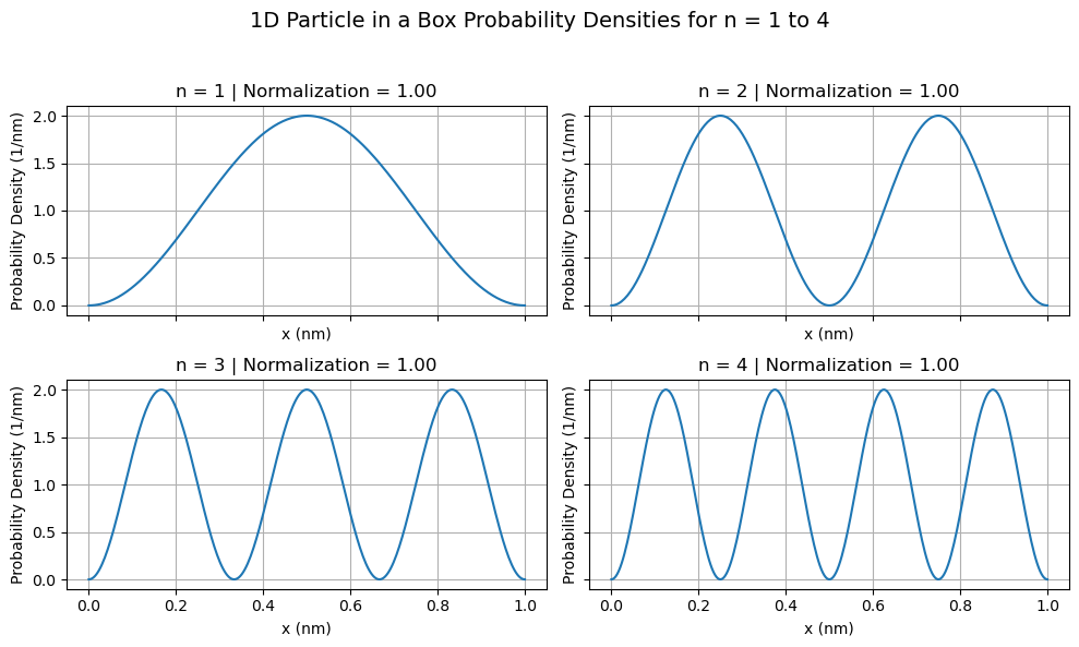
for i, n in enumerate(range(1, 5)):
    y_vals = prob_density_1D(x_vals, n, L)

    # Integrate to verify normalization
    result, _ = quad(lambda x: prob_density_1D(x, n, L), 0, L)
    
    ax = axes[i]
    ax.plot(x_vals, y_vals)
    ax.set_title(f'n = {n} | Normalization = {result:.2f}')
    ax.set_xlabel('x (nm)')
    ax.set_ylabel('Probability Density (1/nm)')
    ax.grid(True)

# Add overall title
fig.suptitle("1D Particle in a Box Probability Densities for n = 1 to 4", fontsize=14)
fig.tight_layout(rect=[0, 0, 1, 0.95])  # Leaves space for the suptitle
plt.show()

2D Box

\[ \psi_{n,m}(x, y) = \sqrt{\frac{4}{L_x L_y}} \sin\left(\frac{n\pi x}{L_x}\right)\sin\left(\frac{m\pi y}{L_y}\right) \]

\[ |\psi_{n,m}(x,y)|^2 = \frac{4}{L_x L_y} \sin^2\left(\frac{n\pi x}{L_x}\right) \sin^2\left(\frac{m\pi y}{L_y}\right) \]

from scipy.integrate import dblquad

def prob_density_2D(x, y, n, m, Lx, Ly):
    norm = 4 / (Lx * Ly)
    return norm * (np.sin(n * np.pi * x / Lx)**2) * (np.sin(m * np.pi * y / Ly)**2)

n, m = 1, 2
Lx, Ly = 1.0, 1.0

# Normalize
result, _ = dblquad(lambda y, x: prob_density_2D(x, y, n, m, Lx, Ly),
                    0, Lx, lambda x: 0, lambda x: Ly)
print(f"2D normalization integral = {result:.6f}")

# Create grid for plotting
x = np.linspace(0, Lx, 200)
y = np.linspace(0, Ly, 200)
X, Y = np.meshgrid(x, y)
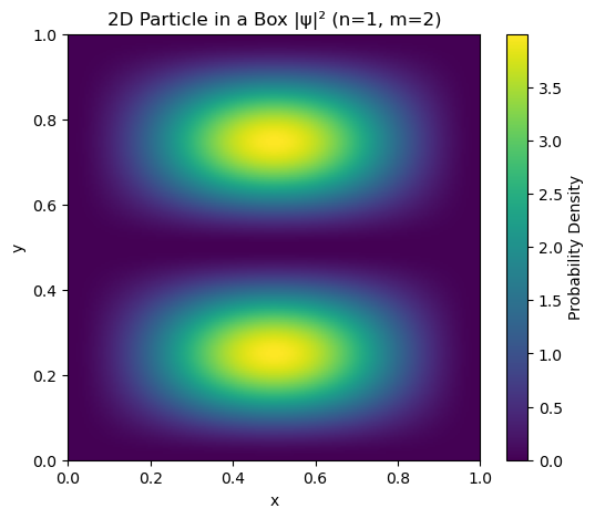
Z = prob_density_2D(X, Y, n, m, Lx, Ly)


# 2D heatmap
plt.figure(figsize=(6, 5))
plt.imshow(Z, extent=[0, Lx, 0, Ly], origin='lower', cmap='viridis', aspect='auto')
plt.colorbar(label='Probability Density')
plt.title(f'2D Particle in a Box |ψ|² (n={n}, m={m})')
plt.xlabel('x')
plt.ylabel('y')
plt.show()

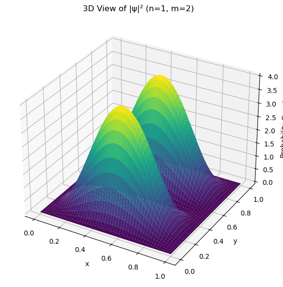
# 3D surface plot
fig = plt.figure(figsize=(8, 6))
ax = fig.add_subplot(111, projection='3d')
ax.plot_surface(X, Y, Z, cmap='viridis', edgecolor='none')
ax.set_title(f'3D View of |ψ|² (n={n}, m={m})')
ax.set_xlabel('x')
ax.set_ylabel('y')
ax.set_zlabel('Probability Density')
plt.tight_layout()
plt.show()

2D normalization integral = 1.000000

import numpy as np
import matplotlib.pyplot as plt
from scipy.integrate import dblquad
from mpl_toolkits.mplot3d import Axes3D  # Required for 3D plotting

# 2D normalized probability density function
def prob_density_2D(x, y, n, m, Lx, Ly):
    norm = 4 / (Lx * Ly)
    return norm * (np.sin(n * np.pi * x / Lx)**2) * (np.sin(m * np.pi * y / Ly)**2)

# Set box size and grid
Lx = Ly = 1.0
x = np.linspace(0, Lx, 100)
y = np.linspace(0, Ly, 100)
X, Y = np.meshgrid(x, y)

# Quantum number pairs
quantum_numbers = [(1, 1), (2, 1), (1, 2), (2, 2)]

# Set up figure
fig = plt.figure(figsize=(12, 10))
for i, (n, m) in enumerate(quantum_numbers):
    Z = prob_density_2D(X, Y, n, m, Lx, Ly)
    
    # Check normalization
    result, _ = dblquad(lambda y, x: prob_density_2D(x, y, n, m, Lx, Ly),
                        0, Lx, lambda x: 0, lambda x: Ly)
    
    ax = fig.add_subplot(2, 2, i+1, projection='3d')
    ax.plot_surface(X, Y, Z, cmap='viridis', edgecolor='k', linewidth=0.2)
    ax.set_title(f'n={n}, m={m} | ∫|ψ|² dA ≈ {result:.2f}')
    ax.set_xlabel('x')
    ax.set_ylabel('y')
    ax.set_zlabel('Probability Density')

fig.suptitle("2D Particle in a Box — Surface Plots of |ψ(x,y)|²", fontsize=16)
plt.tight_layout(rect=[0, 0, 1, 0.95])
plt.show()

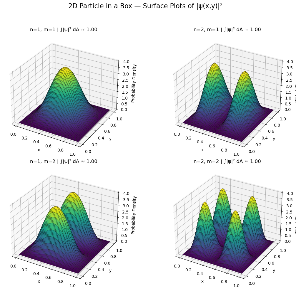
Quantum Numbers	Node Orientation
( n=1, m=1 )	No nodes — ground state
( n=2, m=1 )	Node along ( x = 0.5 )
( n=1, m=2 )	Node along ( y = 0.5 )
( n=2, m=2 )	Nodes along both x and y midpoints

3D Box

\[ \psi_{n,m,l}(x,y,z) = \sqrt{\frac{8}{L_x L_y L_z}} \sin\left(\frac{n\pi x}{L_x}\right)\sin\left(\frac{m\pi y}{L_y}\right)\sin\left(\frac{l\pi z}{L_z}\right) \]

\[ |\psi_{n,m,l}(x,y,z)|^2 = \frac{8}{L_x L_y L_z} \sin^2\left(\frac{n\pi x}{L_x}\right)\sin^2\left(\frac{m\pi y}{L_y}\right)\sin^2\left(\frac{l\pi z}{L_z}\right) \]

import numpy as np
import matplotlib.pyplot as plt
from matplotlib import animation
from IPython.display import HTML

# Quantum numbers and box size
n, m, l = 2, 2, 3
Lx = Ly = Lz = 1.0

# Probability density function
def prob_density_3D(x, y, z):
    norm = 8 / (Lx * Ly * Lz)
    return norm * (np.sin(n * np.pi * x / Lx)**2) * \
                  (np.sin(m * np.pi * y / Ly)**2) * \
                  (np.sin(l * np.pi * z / Lz)**2)

# Create grid
x = np.linspace(0, Lx, 200)
y = np.linspace(0, Ly, 200)
X, Y = np.meshgrid(x, y)
z_vals = np.linspace(0, Lz, 60)
Z_slices = [prob_density_3D(X, Y, z) for z in z_vals]
max_val = np.max(Z_slices)

from scipy.integrate import tplquad
integral_result, error_estimate = tplquad(
    lambda z, y, x: prob_density_3D(x, y, z),
    0, Lx,
    lambda x: 0, lambda x: Ly,
    lambda x, y: 0, lambda x, y: Lz
)
print(f"3D normalization integral = {integral_result:.6f} (error ≈ {error_estimate:.1e})")

# Set up figure
fig, ax = plt.subplots(figsize=(6, 5))
im = ax.imshow(Z_slices[0], extent=[0, Lx, 0, Ly], origin='lower',
               cmap='viridis', vmin=0, vmax=max_val, aspect='auto')
cbar = plt.colorbar(im, ax=ax, label='Probability Density (1/nm³)')
title = ax.set_title("")
ax.set_xlabel("x (nm)")
ax.set_ylabel("y (nm)")

# Animation function
def update(frame):
    im.set_array(Z_slices[frame])
    title.set_text(f"|ψ(x,y,z)|², z = {z_vals[frame]:.2f} nm")
    return im, title

ani = animation.FuncAnimation(fig, update, frames=len(z_vals), interval=100, blit=False)

# Save to GIF (requires ImageMagick) or use mp4 instead
# ani.save("quantum_box.gif", writer="imagemagick")  # Uncomment if ImageMagick is installed

# Save as MP4 using ffmpeg (more reliable)
ani.save("quantum_box.mp4", writer="ffmpeg")

plt.close(fig)  # This prevents the still frame from being shown


# Display inline in notebook
HTML(f"""
<video width="500" controls>
  <source src="quantum_box.mp4" type="video/mp4">
</video>
""")

3D normalization integral = 1.000000 (error ≈ 1.1e-08)

\[ |\psi(x, y, z)|^2 = \frac{8}{L_x L_y L_z} \cdot \sin^2\left(\frac{2\pi x}{L_x}\right) \cdot \sin^2\left(\frac{2\pi y}{L_y}\right) \cdot \sin^2\left(\frac{3\pi z}{L_z}\right) \]

---

Nodal Planes

Each quantum number creates ( n-1 ), ( m-1 ), and ( l-1 ) nodal planes in the respective direction:

Direction	Quantum #	Nodal Planes	Node Locations
x	n = 2	1	\( x = 0.5 \)
y	m = 2	1	\( y = 0.5 \)
z	l = 3	2	\( z = \frac{1}{3}, \frac{2}{3} \)
So we expect 12 regions of particle density

---

Go to the code cell above and change the values of n,m and l. Rerun the code and then see if the updated animation correctly predicts the number of surfaces.

4. Scipy.optimize is used for optimization tasks in Python

common tools are:

• Scalar minimization: Optimize functions of one variable.

• Multivariate minimization: Optimize functions of several variables.

• Curve fitting: Fit models to data.

• Root finding: Find solutions to equations (f(x) = 0).

• Constrained optimization: Optimization with constraints (bounds, equalities, inequalities).

1. Scalar Minimization (Single Variable) | Function | Description | |————————|—————————————————————————| | minimize_scalar() | Finds the minimum of a scalar (1D) function. |

2. Multivariate Minimization (Multiple Variables) | Function | Description | |————————|—————————————————————————| | minimize() | General-purpose minimizer for multivariate functions. | | basinhopping() | Global optimizer that combines local minimization with random perturbation. | | shgo() | Global optimization method using simplicial homology (supports constraints). | | dual_annealing() | Simulated annealing for global optimization. | | differential_evolution() | Evolutionary algorithm for global optimization. |

3. Root Finding (Solving f(x) = 0) | Function | Description | |————————|—————————————————————————| | root_scalar() | Finds the root of a 1D function. | | root() | Finds the root of multivariate systems. | | brentq(), brenth() | Root-finding methods that require a sign change in the interval. | | newton() | Newton-Raphson method for root finding (optionally uses derivative). | | fixed_point() | Solves f(x) = x for fixed points. |

4. Curve Fitting / Least Squares | Function | Description | |————————|—————————————————————————| | curve_fit() | Fits a nonlinear model to data (wraps least_squares). | | least_squares() | Solves nonlinear least-squares problems (general-purpose). |

5. Constrained Optimization | Object / Function | Description | |————————-|—————————————————————————| | Bounds | Specify variable bounds for constraints. | | LinearConstraint | Define constraints of the form Ax <= b. | | NonlinearConstraint | Define nonlinear constraint conditions. |

6. Linear Programming | Function | Description | |————————|—————————————————————————| | linprog() | Solves linear programming problems. |

7. Results and Output | Class | Description | |————————|—————————————————————————| | OptimizeResult | Object returned from most optimizers containing .x, .fun, .success, etc. |

Scalar Minimization

What is the minimum for the following? $\( (x - 2)x (x + 2)^2 \)$

from scipy.optimize import minimize_scalar

def f(x):
    return (x - 2) * x * (x + 2)**2

res = minimize_scalar(f)
print(f"Minimum found at x = {res.x}")
print(f"Minimum function value = {res.fun}")

Minimum found at x = 1.2807764040333458
Minimum function value = -9.914949590828147

import numpy as np
import matplotlib.pyplot as plt
from scipy.optimize import minimize_scalar

# Define the function to minimize
def f(x):
    return (x - 2) * x * (x + 2)**2

# Generate x values for plotting
x_vals = np.linspace(-3, 3, 400)
y_vals = f(x_vals)

# Perform scalar minimization
res = minimize_scalar(f)
x_min = res.x
y_min = res.fun

# Create the plot
plt.figure(figsize=(8, 5))
plt.plot(x_vals, y_vals, label='f(x)', linewidth=2)
plt.plot(x_min, y_min, 'ro', label=f'Minimum at x = {x_min:.2f}')
plt.axvline(x_min, color='r', linestyle='--', alpha=0.6)

# Add function equation to the plot
equation = r"$f(x) = (x - 2) \cdot x \cdot (x + 2)^2$"
plt.text(-2.8, 40, equation, fontsize=12, bbox=dict(facecolor='white', alpha=0.8))

plt.title('Minimizing a Scalar Function with SciPy')
plt.xlabel('x')
plt.ylabel('f(x)')
plt.legend()
plt.grid(True)
plt.tight_layout()
plt.show()
res = minimize_scalar(f)
print(f"Minimum found at x = {res.x}")
print(f"Minimum function value = {res.fun}")

Minimum found at x = 1.2807764040333458
Minimum function value = -9.914949590828147

import numpy as np
import matplotlib.pyplot as plt
from scipy.optimize import minimize_scalar

# Define the function to minimize
def f(x):
    return (x - 2) * x * (x + 2)**2

# Generate x values for plotting
x_vals = np.linspace(-3, 3, 400)
y_vals = f(x_vals)

# Perform scalar minimization
res = minimize_scalar(f)
x_min = res.x
y_min = res.fun

# Create the plot
plt.figure(figsize=(8, 5))
plt.plot(x_vals, y_vals, label='f(x)', linewidth=2)
plt.plot(x_min, y_min, 'ro', label=f"Minimum:\nx = {x_min:.3f}\nf(x) = {y_min:.3f}")
plt.axvline(x_min, color='r', linestyle='--', alpha=0.6)

# Add function equation to the plot
equation = r"$f(x) = (x - 2) \cdot x \cdot (x + 2)^2$"
plt.text(-2.8, 40, equation, fontsize=12, bbox=dict(facecolor='white', alpha=0.8))

plt.title('Minimizing a Scalar Function with SciPy')
plt.xlabel('x')
plt.ylabel('f(x)')
plt.legend()
plt.grid(True)
plt.tight_layout()
plt.show()

# Still print values below graph if you want
print(f"Minimum found at x = {x_min}")
print(f"Minimum function value = {y_min}")

Minimum found at x = 1.2807764040333458
Minimum function value = -9.914949590828147

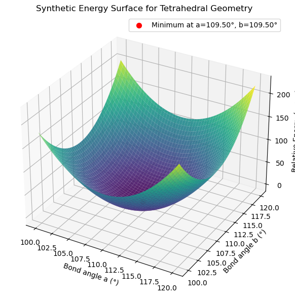
Multivariate Minimization

from scipy.optimize import minimize
import numpy as np

# Example: energy surface with two bond angles
def energy(x):
    a, b = x
    return (a - 109.5)**2 + (b - 109.5)**2  # Deviation from ideal tetrahedral angle

res = minimize(energy, x0=[100, 100])
print(f"Optimal angles = {res.x}")

Optimal angles = [109.50000066 109.50000066]

import numpy as np
import matplotlib.pyplot as plt
from scipy.optimize import minimize

# Define the energy function
def energy(x):
    a, b = x
    return (a - 109.5)**2 + (b - 109.5)**2

# Perform the minimization
res = minimize(energy, x0=[100, 100])
a_min, b_min = res.x

# Create a grid for visualization
a = np.linspace(100, 120, 100)
b = np.linspace(100, 120, 100)
A, B = np.meshgrid(a, b)
Z = (A - 109.5)**2 + (B - 109.5)**2

# Plot the energy surface
fig = plt.figure(figsize=(10, 6))
ax = fig.add_subplot(111, projection='3d')
surf = ax.plot_surface(A, B, Z, cmap='viridis', edgecolor='none', alpha=0.9)

# More descriptive legend
label = f'Minimum at a={a_min:.2f}°, b={b_min:.2f}°'
ax.scatter(a_min, b_min, energy([a_min, b_min]), color='red', s=50, label=label)

# Axis labels and title
ax.set_xlabel('Bond angle a (°)')
ax.set_ylabel('Bond angle b (°)')
ax.set_zlabel('Relative Energy (proxy)')
ax.set_title('Synthetic Energy Surface for Tetrahedral Geometry')
ax.legend()

plt.tight_layout()
plt.show()

Root Finding

This script models the ICE table (Initial, Change, Equilibrium) for acetic acid dissociation:

\[ \text{CH}_3\text{COOH} \rightleftharpoons \text{CH}_3\text{COO}^- + \text{H}^+ \]

You’re solving for x = [H⁺] at equilibrium using the Ka expression:

\[ K_a = \frac{[H^+]^2}{[CH_3COOH]_{\text{initial}} - [H^+]} \]

Here:

• \( K_a = 1.8 \times 10^{-5} \)

• Initial acetic acid concentration = 0.1 M

• The equation becomes:

  Ka - (x**2 / (0.1 - x)) = 0
  

from scipy.optimize import root_scalar

def equilibrium(x):
    Ka = 1.8e-5  # Acetic acid Ka
    return Ka - (x**2 / (0.1 - x))  # ICE table expression

res = root_scalar(equilibrium, bracket=[0, 0.09])
print(f"[H⁺] at equilibrium = {res.root:.5f} M")

[H⁺] at equilibrium = 0.00133 M

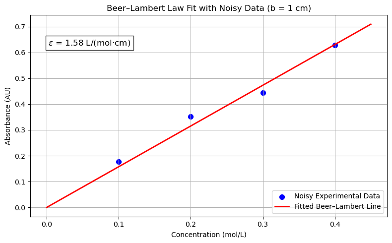
Curve Fitting (Beer-Lambert law)

import numpy as np
import matplotlib.pyplot as plt
from scipy.optimize import curve_fit

# Define Beer–Lambert Law with fixed path length b = 1 cm
def beer_lambert(c, epsilon):
    b = 1  # Path length in cm
    return epsilon * b * c

# Original concentration (mol/L) and absorbance data
concentration = np.array([0.1, 0.2, 0.3, 0.4])
true_absorbance = np.array([0.15, 0.31, 0.45, 0.61])  # True absorbance data

# Add random noise to the absorbance data
noise = np.random.normal(0, 0.02, size=concentration.shape)  # Mean = 0, Std = 0.02
noisy_absorbance = true_absorbance + noise

# Fit the curve to determine epsilon
params, _ = curve_fit(beer_lambert, concentration, noisy_absorbance)
epsilon = params[0]

# Print the fitted molar absorptivity
print(f"Epsilon (molar absorptivity) = {epsilon:.3f} L/(mol·cm)")

# Generate fit line
c_fit = np.linspace(0, 0.45, 100)
a_fit = beer_lambert(c_fit, epsilon)

# Plot the data and fit
plt.figure(figsize=(8, 5))
plt.scatter(concentration, noisy_absorbance, color='blue', label='Noisy Experimental Data', s=50)
plt.plot(c_fit, a_fit, 'r-', label='Fitted Beer–Lambert Line', linewidth=2)
plt.title('Beer–Lambert Law Fit with Noisy Data (b = 1 cm)')
plt.xlabel('Concentration (mol/L)')
plt.ylabel('Absorbance (AU)')
plt.legend()
plt.grid(True)

# Annotate the plot with the fitted epsilon value without an arrow
annotation_text = fr"$\epsilon$ = {epsilon:.2f} L/(mol·cm)"
plt.annotate(annotation_text, xy=(0.05, 0.85), xycoords='axes fraction',
             fontsize=12, bbox=dict(facecolor='white', alpha=0.8))

plt.tight_layout()
plt.show()

Epsilon (molar absorptivity) = 1.576 L/(mol·cm)

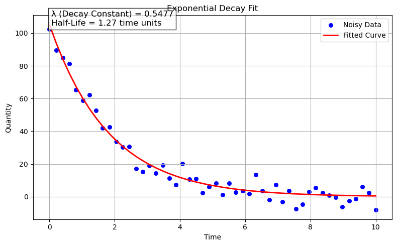
import numpy as np
import matplotlib.pyplot as plt
from scipy.optimize import curve_fit

# Define the exponential decay function
def decay_function(t, N0, lambda_):
    return N0 * np.exp(-lambda_ * t)

# Generate synthetic data
np.random.seed(42)  # For reproducibility
time = np.linspace(0, 10, num=50)  # Time from 0 to 10 units
true_N0 = 100  # True initial quantity
true_lambda = 0.5  # True decay constant
noise = np.random.normal(0, 5, size=time.shape)  # Gaussian noise
quantity = decay_function(time, true_N0, true_lambda) + noise  # Noisy measurements

# Fit the data to the exponential decay function
popt, pcov = curve_fit(decay_function, time, quantity, p0=(true_N0, true_lambda))
fitted_N0, fitted_lambda = popt

# Calculate the half-life
half_life = np.log(2) / fitted_lambda

# Print the fitted parameters
print(f"Fitted Initial Quantity (N0): {fitted_N0:.2f}")
print(f"Fitted Decay Constant (lambda): {fitted_lambda:.4f}")
print(f"Calculated Half-Life: {half_life:.2f} time units")

# Plot the data and the fitted curve
plt.figure(figsize=(8, 5))
plt.scatter(time, quantity, color='blue', label='Noisy Data', s=30)
plt.plot(time, decay_function(time, fitted_N0, fitted_lambda), 'r-', label='Fitted Curve', linewidth=2)
plt.title('Exponential Decay Fit')
plt.xlabel('Time')
plt.ylabel('Quantity')
plt.legend()
plt.grid(True)

# Annotate the plot with the decay constant and half-life
annotation_text = f"λ (Decay Constant) = {fitted_lambda:.4f}\nHalf-Life = {half_life:.2f} time units"
plt.annotate(annotation_text, xy=(0.05, 0.95), xycoords='axes fraction',
             fontsize=12, bbox=dict(facecolor='white', alpha=0.8))

plt.tight_layout()
plt.show()

Fitted Initial Quantity (N0): 105.25
Fitted Decay Constant (lambda): 0.5477
Calculated Half-Life: 1.27 time units

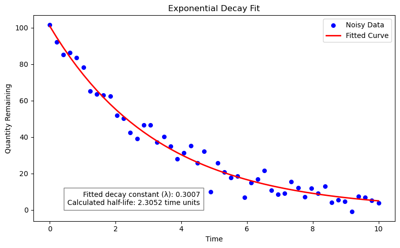
import numpy as np
import matplotlib.pyplot as plt
from scipy.optimize import curve_fit

# Define the exponential decay function
def decay_function(t, N0, lambda_):
    return N0 * np.exp(-lambda_ * t)

# Generate synthetic data
#np.random.seed(444)  # For reproducibility
time = np.linspace(0, 10, num=50)  # Time from 0 to 10 units
true_N0 = 100  # True initial quantity
true_lambda = 0.3  # True decay constant
decay_data = decay_function(time, true_N0, true_lambda)
noise = np.random.normal(0, 5, size=decay_data.shape)  # Add some noise
noisy_decay_data = decay_data + noise

# Perform curve fitting
popt, pcov = curve_fit(decay_function, time, noisy_decay_data, p0=(true_N0, true_lambda))
fitted_N0, fitted_lambda = popt

# Calculate half-life
half_life = np.log(2) / fitted_lambda

# Print the decay constant and half-life
print(f"Fitted decay constant (lambda): {fitted_lambda:.4f}")
print(f"Calculated half-life: {half_life:.4f} time units")

# Plot the data and the fitted curve
plt.figure(figsize=(8, 5))
plt.scatter(time, noisy_decay_data, color='blue', label='Noisy Data', s=30)
plt.plot(time, decay_function(time, *popt), 'r-', label='Fitted Curve', linewidth=2)
plt.title('Exponential Decay Fit')
plt.xlabel('Time')
plt.ylabel('Quantity Remaining')
plt.legend()
plt.grid(False)  # Remove grid lines

# Add annotation below the x-axis label
annotation_text = f"Fitted decay constant (λ): {fitted_lambda:.4f}\nCalculated half-life: {half_life:.4f} time units"
plt.figtext(0.5, 0.18, annotation_text, ha="right", fontsize=10, bbox={"facecolor": "white", "alpha": 0.5, "pad": 5})

plt.tight_layout()
plt.show()

Fitted decay constant (lambda): 0.3007
Calculated half-life: 2.3052 time units

import numpy as np
import matplotlib.pyplot as plt
from scipy.optimize import curve_fit

# Step 1: Generate synthetic data
# --------------------------------
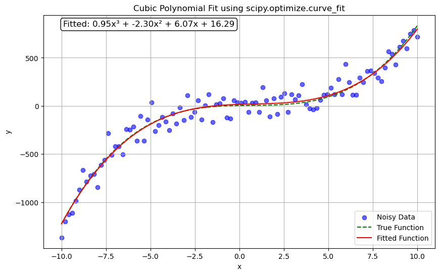
# Define true coefficients for the cubic polynomial: y = a*x^3 + b*x^2 + c*x + d
a_true, b_true, c_true, d_true = 1.0, -2.0, 3.0, 4.0

# Generate 100 x-values evenly spaced between -10 and 10
x_data = np.linspace(-10, 10, 100)

# Compute corresponding y-values using the true polynomial coefficients
y_true = a_true * x_data**3 + b_true * x_data**2 + c_true * x_data + d_true

# Add normally distributed noise to the y-values to simulate real-world data
noise = np.random.normal(0, 100, size=x_data.size)
y_data = y_true + noise

# Step 2: Define the cubic polynomial model function
# ---------------------------------------------------
def cubic_model(x, a, b, c, d):
    """
    Cubic polynomial model: y = a*x^3 + b*x^2 + c*x + d
    """
    return a * x**3 + b * x**2 + c * x + d

# Step 3: Perform curve fitting using scipy's curve_fit
# ------------------------------------------------------
# Provide an initial guess for the parameters (optional but can aid convergence)
initial_guess = [1.0, 1.0, 1.0, 1.0]

# Use curve_fit to find the optimal parameters that fit the cubic model to the data
popt, pcov = curve_fit(cubic_model, x_data, y_data, p0=initial_guess)

# Extract the optimal parameters
a_fit, b_fit, c_fit, d_fit = popt

# Step 4: Visualize the original data and the fitted curve
# ---------------------------------------------------------
plt.figure(figsize=(10, 6))

# Scatter plot of the noisy data
plt.scatter(x_data, y_data, color='blue', label='Noisy Data', alpha=0.6)

# Plot of the true underlying cubic function (without noise)
plt.plot(x_data, y_true, color='green', linestyle='--', label='True Function')

# Plot of the fitted cubic function using the optimized parameters
plt.plot(x_data, cubic_model(x_data, *popt), color='red', label='Fitted Function')

# Annotate the plot with the fitted equation
equation = f'Fitted: {a_fit:.2f}x³ + {b_fit:.2f}x² + {c_fit:.2f}x + {d_fit:.2f}'
plt.annotate(equation, xy=(0.05, 0.95), xycoords='axes fraction', fontsize=12,
             bbox=dict(boxstyle="round,pad=0.3", edgecolor='black', facecolor='white'))

# Add labels, title, legend, and grid
plt.xlabel('x')
plt.ylabel('y')
plt.title('Cubic Polynomial Fit using scipy.optimize.curve_fit')
plt.legend()
plt.grid(True)

# Display the plot
plt.show()

Understanding the polynomial fit

Lets focus on this section here:

# Step 3: Perform curve fitting using scipy's curve_fit
# ------------------------------------------------------

# Provide an initial guess for the parameters (optional but can aid convergence)
initial_guess = [1.0, 1.0, 1.0, 1.0]

# Use curve_fit to find the optimal parameters that fit the cubic model to the data
popt, pcov = curve_fit(cubic_model, x_data, y_data, p0=initial_guess)

# Extract the optimal parameters
a_fit, b_fit, c_fit, d_fit = popt

1. Initial Guess (p0):

   • The initial_guess provides starting values for the parameters ( a ), ( b ), ( c ), and ( d ) in your cubic model. While curve_fit can often determine reasonable starting points on its own, supplying an initial guess can significantly enhance the convergence and accuracy of the fitting process, especially for complex models.

   • In non-linear curve fitting, the optimization algorithm searches for the set of parameters that minimize the difference between your model and the data. Providing a good initial guess helps the algorithm start closer to the optimal solution, reducing computation time and the risk of converging to a local minimum instead of the global minimum.

   • If you have prior knowledge or intuition about the parameter values based on the data’s nature or previous experiments, you can set initial_guess accordingly. If not, starting with generic values like [1.0, 1.0, 1.0, 1.0] is common, but be aware that poor initial guesses can lead to slow convergence or fitting failures.

2. Curve Fitting with curve_fit:

   • Function Call:curve_fit is called with the following arguments:

     • cubic_model: Your defined function representing the cubic relationship ( y = ax^3 + bx^2 + cx + d ).

     • x_data: The array of independent variable data points.

     • y_data: The array of dependent variable data points.

     • p0=initial_guess: The initial guess for the parameters.

   • curve_fit uses non-linear least squares to fit the cubic_model to the data. It adjusts the parameters ( a ), ( b ), ( c ), and ( d ) to minimize the sum of the squared residuals (the differences between the observed and predicted values).

   • Outputs:

     • popt (Optimal Parameters): An array containing the optimal values for the parameters ( a ), ( b ), ( c ), and ( d ) that best fit the data.

     • pcov (Covariance Matrix): The estimated covariance matrix of popt. The diagonal elements provide the variance of each parameter estimate, which can be used to compute standard errors.

3. Extracting Optimal Parameters:

   • Assignment: The optimal parameters are extracted from popt and assigned to a_fit, b_fit, c_fit, and d_fit. These represent the best estimates for the coefficients in your cubic model.

Constrained Optimization

We aim to find the radius \( r \) and height \( h \) of a cylinder that minimize the surface area, given a fixed volume \( V \). The surface area \( A \) of a cylinder is given by:

\[ A = 2\pi r^2 + 2\pi r h \]

The volume constraint is: $\( V = \pi r^2 h \)$

We’ll use Python’s scipy.optimize module to perform this constrained optimization. The steps include:

1. Define the Objective Function: The surface area to be minimized.

2. Set Up the Constraint: The volume must remain constant.

3. Provide an Initial Guess: Starting values for ( r ) and ( h ).

4. Perform the Optimization: Using scipy.optimize.minimize with the Sequential Least Squares Programming (SLSQP) method, which handles constraints effectively.

import numpy as np
from scipy.optimize import minimize

# Given volume in cubic centimeters
V = 1000  # cm³

# Objective function: Surface area of the cylinder
def surface_area(x):
    r, h = x
    return 2 * np.pi * r**2 + 2 * np.pi * r * h

# Constraint: Volume of the cylinder remains constant
def volume_constraint(x):
    r, h = x
    return np.pi * r**2 * h - V

# Initial guess: radius and height
initial_guess = [5, 10]  # Arbitrary starting values

# Bounds: radius and height must be positive
bounds = [(0.1, None), (0.1, None)]  # Preventing zero or negative dimensions

# Define the constraint in the form required by 'minimize'
constraint = {'type': 'eq', 'fun': volume_constraint}

# Perform the optimization
result = minimize(surface_area, initial_guess, method='SLSQP', bounds=bounds, constraints=constraint)

# Extract the optimized radius and height
optimized_radius, optimized_height = result.x

# Display the results
print(f"Optimized Radius: {optimized_radius:.2f} cm")
print(f"Optimized Height: {optimized_height:.2f} cm")
print(f"Minimum Surface Area: {result.fun:.2f} cm²")

Optimized Radius: 5.52 cm
Optimized Height: 10.43 cm
Minimum Surface Area: 553.79 cm²

Explanation:

• Objective Function (surface_area): Calculates the total surface area of the cylinder based on radius ( r ) and height ( h ).

• Constraint (volume_constraint): Ensures that the product ( \pi r^2 h ) equals the specified volume ( V ).

• Initial Guess: Provides starting values for ( r ) and ( h ) to initiate the optimization process.

• Bounds: Sets lower limits for ( r ) and ( h ) to prevent non-physical negative or zero dimensions.

• Optimization Method: Utilizes the SLSQP algorithm, suitable for problems with equality constraints.

Acknowledgements

This content was developed with assistance from Perplexity AI and Chat GPT. Multiple queries were made during the Fall 2024 and the Spring 2025.